7 Day 6
Announcements
Homework 2 point recovery
Videos
Review
- Population Mean
\[\mu = {1 \over N}\sum\limits_{i=1}^Nx_i\] \[\mu = {\sum\limits_{i=1}^Nx_i\over N}\]
- Sample Mean
\[\bar{x} = {1 \over n}\sum\limits_{i=1}^nx_i\]
\[\bar{x} = {\sum\limits_{i=1}^nx_i\over n}\]
- Spread of data
- Range
\[Range = Max - Min\]
Variance
- Population variance (denoted \(\sigma^2\)):
\[\sigma^2 = {{{\sum\limits_{i=1}^N}(x_i-\mu)^2}\over N}\]
- Sample variance (denoted \(s^2\)):
\[s^2 = {{{\sum\limits_{i=1}^n}(x_i-\bar{x})^2}\over (n-1)}\]
- Standard Deviation
\(\sqrt{\sigma^2}=\sigma \rightarrow Population \ Standard \ Deviation\)$
\[\sqrt{s^2}=s \rightarrow Sample \ Standard \ Deviation\]
- What is the variance and standard deviation of the data below?
| Battery | A | B | C | D | E | F |
| Lifespan | 3 | 4 | 6 | 5 | 4 | 2 |
Empirical Rule
Many data sets has a single peak in the center and an approximately symmetric shape
- We call this a bell-shape
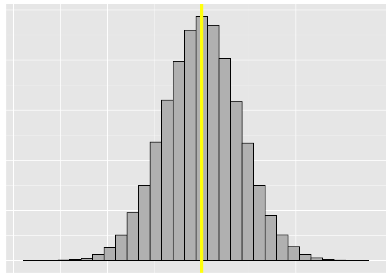
When we see this distribution we can use standard deviation to describe how much of the data is within a certain range of the mean
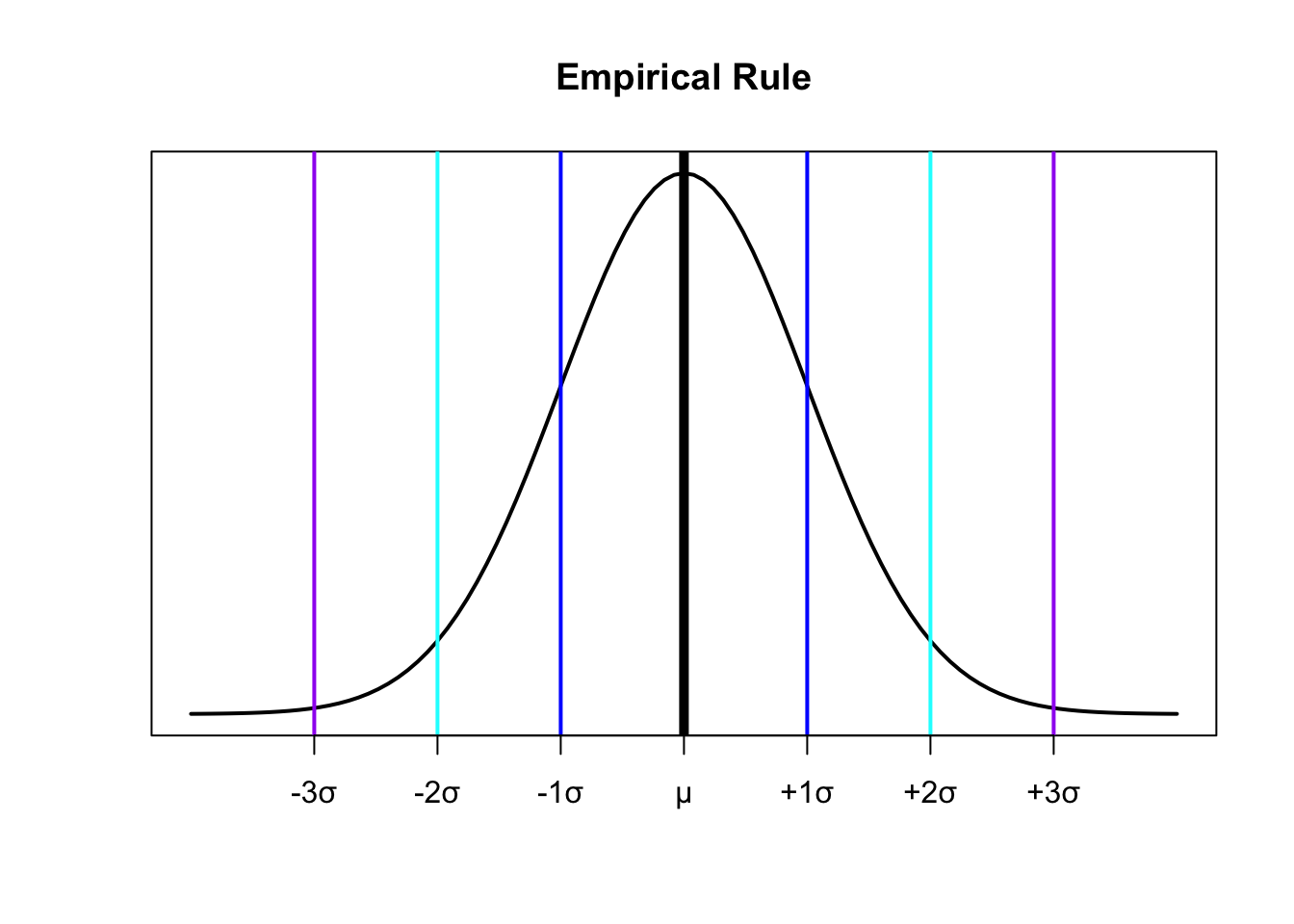
The Empirical Rule
For a population that has an approximately bell-shaped distribution:
\(\approx 68\%\) of the data is within ONE standard deviation of the mean
\[\approx 68\% = \begin{cases} \mu - \sigma \\ \mu + \sigma \end{cases}\]
- \(\approx 95\%\)$ of the data is within TWO standard deviations of the mean
\[\approx 95\% = \begin{cases} \mu - 2\sigma \\ \mu + 2\sigma \end{cases}\]
- \(\approx\) All or almost all of the data is within THREE standard deviations of the mean
\[\approx 100\% = \begin{cases} \mu - 3\sigma \\ \mu + 3\sigma \end{cases}\]
Practice: Empirical Rule
A large class of 200 students took an exam. The scores had sample mean \(\bar{x} = 65\) and sample standard deviation \(s = 10\). The histogram is approximately bell-shaped.
Find an interval that is likely to contain approximately 68% of the scores.
Approximately what percentage of the scores were between 45 and 85?
Approximately how many students had scores between 45 and 85?
Measures of Position
Suppose we have a man who’s \(73\) inches tall and a woman who’s \(68\) inches tall
We have the tools to say how different they are from each other
But how can we say who’s more different from their specific group?
We need to define a way to look at differences relative to groups
This is referred to as position
We’ll develop three general measures of it:
z-scores
percentiles
quartiles
z-scores
Let \(x\) be a value from a population with mean \(\mu\)
- The z-score is:
\[z={x-\mu \over \sigma}\]
- For a sample:
\[z={x-\bar{x} \over s}\]
Suppose you score \(x=75\) on Exam 1. The class average on Exam 1 is \(80\) with a standard deviation of 5. The \(z\)-score of your exam is:
\[z={75-80 \over 5}=-1\]
Population:
\[z={x-\mu \over \sigma}\]
Sample:
\[z={x-\bar{x} \over s}\]
A \(z\)-score data value \(x\) is the number of standard deviations \(x\) is from the mean of the data set
\(z < 0 \Rightarrow\) the value of \(x\) is less than the mean
\(z = 0 \Rightarrow\) the value of \(x\) is equal to the mean
\(z > 0 \Rightarrow\) the value of \(x\) is greater than the mean
In our example:
\(x=75\)
\(z=-1\)
Note: this measure is unitless
Example: z-score calculation
The mean height for adult men is \(\mu=69.4\) inches, with a standard deviation of \(\sigma = 3.1\) inches.
The mean height for adult women is \(\mu=63.8\) inches, with a standard deviation of \(\sigma = 2.8\) inches
Who is taller relative to their gender, a man 73 inches tall or a woman 68 inches tall? Use z-scores to answer this.
\[z={x-\mu \over \sigma}\]
z-scores and the Empirical Rule
Recall the Empirical Rule:
\(\approx 68\%\) of the data will be between \(\mu - \sigma\) and \(\mu + \sigma\)
\(\approx 95\%\) of the data will be between \(\mu - 2\sigma\) and \(\mu + 2\sigma\)
\(\approx 99.9\%\) of the data will be between \(\mu - 3\sigma\) and \(\mu + 3\sigma\)
With z-scores:
\(\approx 68\%\) of the data will be between \(z=-1\) and \(z=1\)
\(\approx 95\%\) of the data will be between \(z=-2\) and \(z=2\)
\(\approx 100\%\) of the data will be between \(z=-3\) and \(z=3\)
Both of these imply a bell-shaped distribution
Example: Empirical Approximation
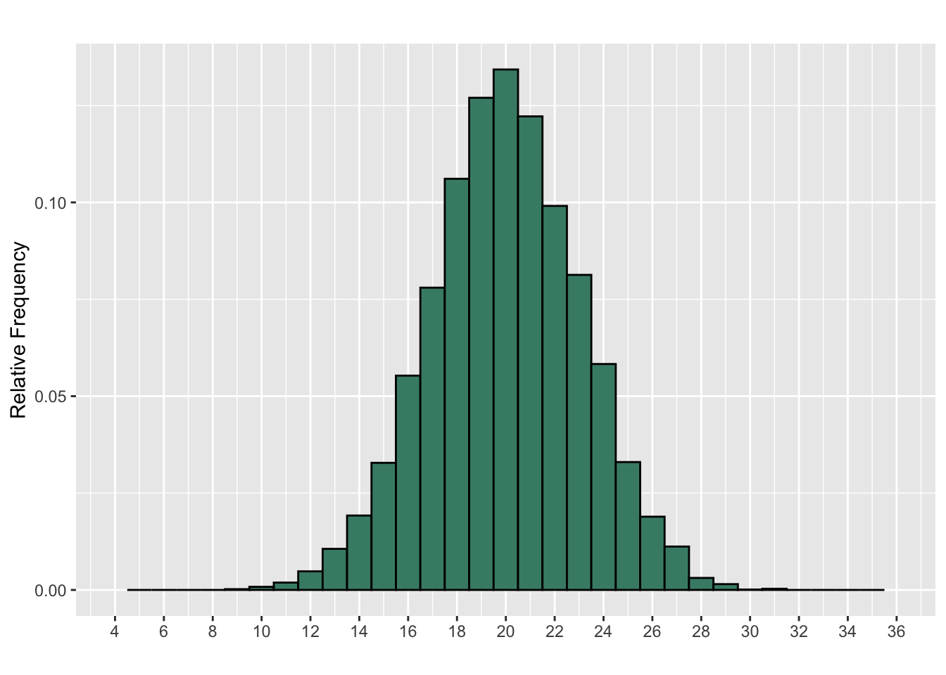
A data set has a mean of 20 and a standard deviation of 3. A histogram for the data is shown below.
Is it appropriate to use the Empirical Rule to approximate the proportion of the data between 14 and 26? If so, find the approximation. If not, explain why not.
Quartiles
Every data set has three quartiles:
\(1^{st}\) quartile, denoted \(\textbf{Q}_1\) separates the lowest \(25\%\) of the data from the highest \(75\%\)
\(2^{nd}\) quartile, denoted \(\textbf{Q}_2\) separates the lowest \(50\%\) of the data from the highest \(50\%\) (\(Q_2 = Median\))
\(3^{rd}\) quartile, denoted \(\textbf{Q}_3\) separates the lowest \(75\%\) of the data from the highest \(25\%\)
- The quartiles of the below data set of size \(n=8\):
\[1 \ \ 2 \ \ 2 \ \ 3 \ \ 4 \ \ 5 \ \ 7 \ \ 12\] \(Q_1\) = 2
\(Q_2\) = 3.5 (Median)
\(Q_3\) = 6
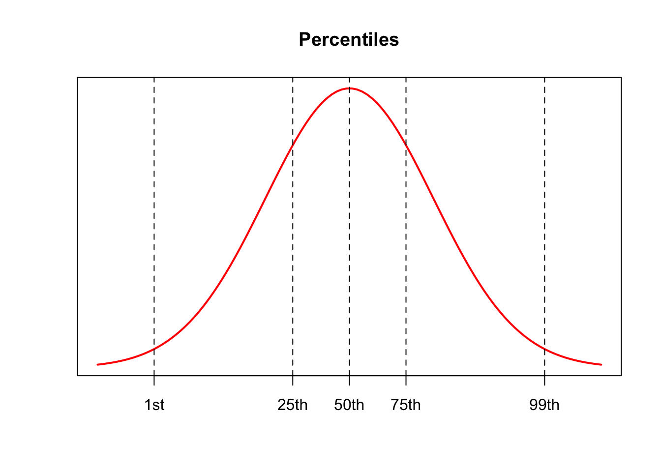
Percentiles
For a number \(p\) between \(1\) and \(99\), the \(p^{th}\) percentile separates the lowest \(p\%\) of the data from the highest \((100-p)\%\)
Quartiles separate data into \(4\) parts
- Each part is \(\approx 25\%\) of the data
Percentiles divide the data set into \(100\) parts
Procedure for Computing Percentiles or Quartiles
Arrange the data in increasing order
Let \(n\) be the number of values in the data set. For the \(p^{th}\) percentile, compute the value:
\[L={p\over 100}*n\]
- If \(L\) is a whole number, the \(p^{th}\) percentile is the average of the number in position \(L\) and the number in position \(L+1\)
- If \(L\) is not a whole number, round it up the the next higher whole number. The \(p^{th}\) percentile is the number in the position corresponding to the rounded-up value
Example 3: Quartiles
Below is a table of scores students received on a quiz in an introductory statistics course.
Find \(Q_1\), \(Q_2\), and \(Q_3\) of the scores:
| Individual | Score | |
|---|---|---|
| 1 | 7 | 10 |
| 2 | 25 | 6 |
| 3 | 30 | 9 |
| 4 | 21 | 9 |
| 5 | 12 | 10 |
| 6 | 8 | 3 |
| 7 | 27 | 8 |
| 10 | 24 | 10 |
| 11 | 19 | 7 |
| 12 | 5 | 6 |
| 13 | 17 | 10 |
| 14 | 22 | 8 |
| 15 | 23 | 9 |
| 16 | 3 | 10 |
| 17 | 1 | 10 |
| 18 | 10 | 10 |
| 19 | 20 | 4 |
| 20 | 16 | 2 |
| 21 | 15 | 9 |
| 22 | 4 | 8 |
| 23 | 14 | 1 |
| 25 | 29 | 8 |
| 26 | 28 | 10 |
| 27 | 6 | 9 |
| 28 | 26 | 6 |
| 29 | 32 | 10 |
| 30 | 13 | 7 |
| 31 | 18 | 6 |
| 32 | 31 | 1 |
| 33 | 2 | 7 |
| 35 | 11 | 9 |
| 37 | 9 | 5 |
Five-Number Summary
The five-number summary is a set of five measures of position computed from a data set. The summary consists of:
\[Min \ \ \ \ \ Q_1 \ \ \ \ \ Median \ \ \ \ \ Q_3 \ \ \ \ \ Max\]
- Below is a table of exam scores from the same class:
| Row_1 | 83 | 72 | 67 | 55 | 53 | 77 | 69 | 84 | 83 | 74 | 60 | 69 | 82 | 81 | 80 |
| Row_2 | 67 | 91 | 78 | 81 | 90 | 79 | 86 | 75 | 75 | 84 | 76 | 81 | 73 | 70 | 79 |
The five number summary is:
| Metric | Min | Q1 | Median | Q3 | Max |
| Value | 53 | 70 | 78 | 82 | 91 |
How does a new value of 86 compare to the exam scores?
- \(Q_3 < 86 < Max \Rightarrow 86\) is greater than \(75\%\) of the exam scores but is not the largest
What about 74?
- \(Q_1 < 74 < Median \Rightarrow 74\) is greater than \(25\%\) of the exam scores, but less than half of the exams
Outliers
An outlier is a value that is considerably large or smaller than most of the values in a data set
What do you do with outliers?
If it’s a mistake/type/bad measure, ideally fix it
If you can’t fix it, chuck it
If it’s a valid observation, you keep it in the data
You keep outliers if they’re valid observations
- Keep outliers if they’re valid
Resistant metrics
- How do you find outliers?
Interquartile Range (IQR)
The IQR is a measure of spread that is often used to detect outliers
Take the difference between \(Q_1\) and \(Q_3\):
\[IQR = Q_3 - Q_1\]
- Notice the IQR contains the middle \(50\%\) of the data
- To find outliers with the IQR we use the IQR Method
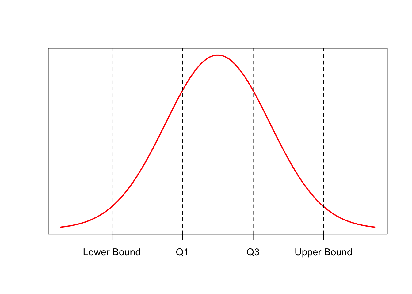
- Define outlier boundaries:
\[Lower \ Outlier \ Boundary = Q_1 - 1.5*IQR\] \[Upper \ Outlier \ Boundary = Q_3 + 1.5*IQR\]
- Check to see if any data is outside of these boundaries:
\[Upper \ Boundary < x < Lower \ Boundary\]
- Recall our five-number summary of the exam data:
| Metric | Min | Q1 | Median | Q3 | Max |
| Value | 53 | 70 | 78 | 82 | 91 |
- The IQR for the dataset is:
\[IQR = Q_3 - Q_1 = 82 - 70 = 12\]
- Defining the outlier boundaries:
\[Q_3 + 1.5*IQR = 82 + (1.5*12)=100\]
\[Q_1 - 1.5*IQR = 70-(1.5*12)=52\]
Any value in the dataset \(>100\) or \(<52\) is an outlier
Since \(Min = 53 > 52\) and \(Max = 91 < 100\) there are no outliers in the dataset
Example: 5 Number Summary and Outliers
Jamie drives to work every weekday morning, She keeps track of the time it takes, in minutes, for \(35\) days. The results are below:
| 15 | 17 | 17 | 17 | 17 |
| 18 | 19 | 19 | 19 | 19 |
| 19 | 19 | 20 | 20 | 20 |
| 20 | 20 | 21 | 21 | 21 |
| 21 | 21 | 21 | 21 | 21 |
| 21 | 22 | 23 | 23 | 24 |
| 26 | 31 | 36 | 38 | 39 |
- Find the five-number summary:
\[Min \ \ \ \ \ Q_1 \ \ \ \ \ Median \ \ \ \ \ Q_3 \ \ \ \ \ Max\]
- List all the values, if any, that are classified as outliers:
- Go away