14 Day 13
Announcements
Homework corrections grading crunch
- Get them in before Friday if you want an updated grade before \(\approx 2\) weeks
Exam performance metrics
Please stay ahead on homeworks
- This helps both of us
Office hours are cancelled for today
- Feel free to come to my Thursday office hours (9-10 AM)
Review
Random variable (shorthand: r.v.):
- A rule for assigning a numerical value to each outcome of a random experiment
Flip a fair coin \(3\) independent times
Let r.v. \(X=\{\text{the number of tails observed}\}\)
\[S=\{HHH,HHT,HTH,THH,HTT,THT,TTH,TTT\}\]
The r.v. has its own sample space or support
- Support the set of possible values it can be
The support of \(X\) is \(S_X=\{0,1,2,3\}\)
\[x=\text{the value after the experiement has been performed (not random)}\]
\[X=\text{the value before the experiement has been performed (still random)}\]
\[P(X=x)\ \text{means the probability that r.v.} \ X \ \text{is equal to possible value} \ x\]
\[P(X>x) \ \text{means the probability that r.v.} \ X \ \text{is greater than possible value} \ x\]
Random Variable Types
Discrete
- The number of possible values in the support is finite or countably infinite
Let \(Y=\{\text{The number of fish in a pond}\}\)
The support of \(Y\), \(S_Y=\{0,1,2,...\}\)
Can I have half a fish? Technically yes. But half a fish isn’t biologically logical.
If partial counts feel arbitrary then you’re more than likely working with a discrete variable
I can hypothetically have infinite fish, but the realized value will always be a whole number
Probability Distributions
The form of a r.v.’s probability distribution depends on whether it is continuous or discrete
For a discrete random variable the probability distribution is often a list of all possible values the r.v. can take and their corresponding probabilities of occurrence
Discrete probability distributions satisfy the following two properties:
\[i. \ 0 \le P(X=x) \le 1\]
\[ii. \ \sum_x P(X=x)=1\]
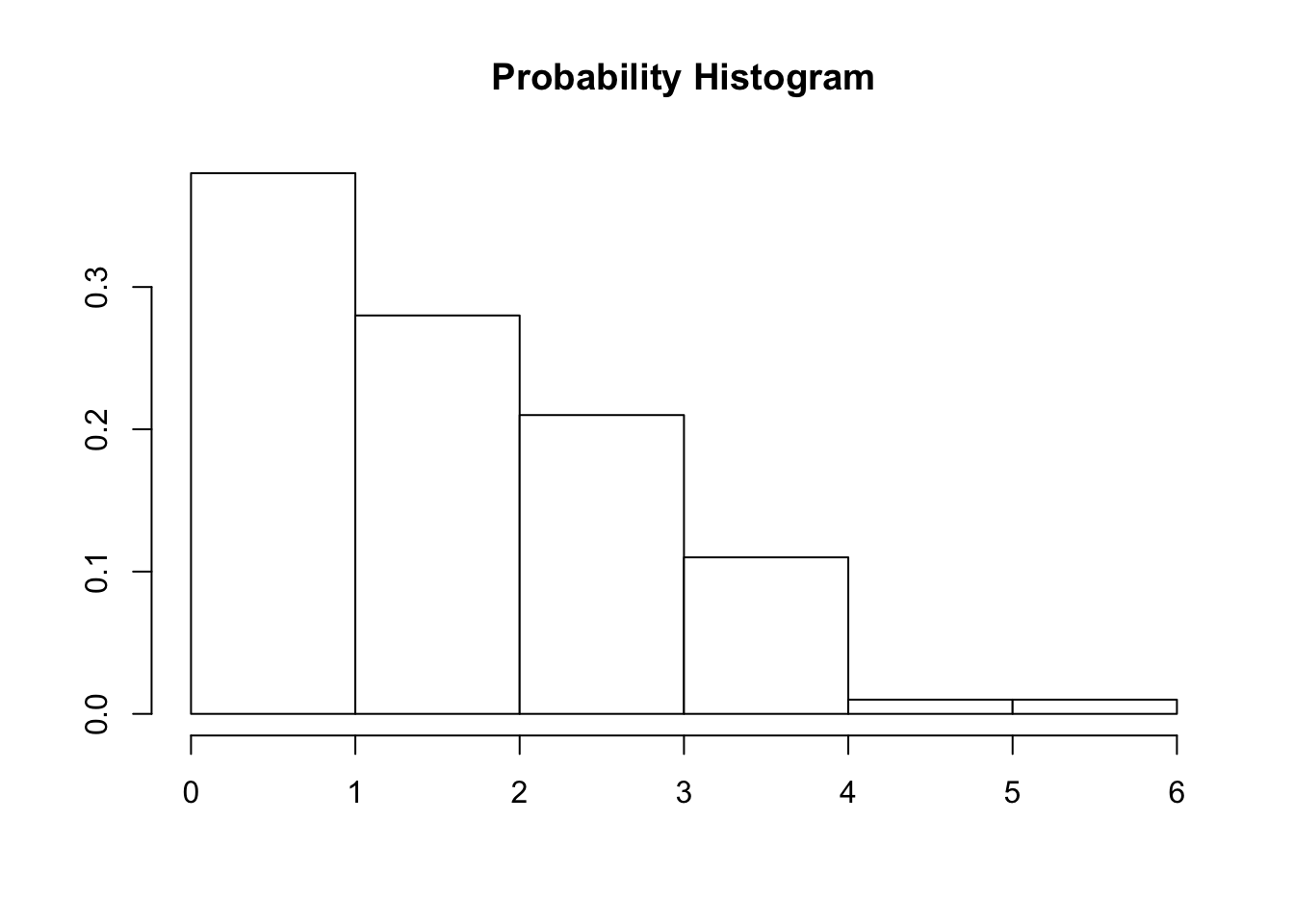
We can draw a histogram so that the area of each bar above a given possible value of a r.v. is equal to it’s probability of occurrence
Probability Distribution Mean
For a discrete probability distribution of r.v. \(X\), the mean is given by:
\[E(X)=\mu=\sum_x xP(X=x)\]
- We call this “the weighted sum of all probabilities of \(x\)”
\(X=\{\text{number of customers in a line at the express checkout counter}\}\)
\[ \begin{array}{|c|c|c|c|c|c|c|} \hline x & 0 & 1 & 2 & 3 & 4 & 5 \\ \hline P(X = x) & 0.4 & 0.2 & 0.15 & 0.1 & 0.1 & 0.05 \\ \hline \end{array} \]
\[\mu_X=\sum_x xP(X=x)\]
\[=0(0.4)+1(0.2)+2(0.15)+3(0.1)+4(0.1)+5(0.05)=1.45\]
- This is the “average in the long run”
Probability Distribution Variance
Denoting the variance of discrete r.v. \(X\):
\[\sigma^2_X \ \ \ \ \ \text{or} \ \ \ \ \ Var(X)\]
The general formula for the variance of r.v. \(X\):
\[\sigma^2=\sum_x (x-\mu)^2 P(X=x)\]
\[=(0-1.45)^2(0.4)+(1-1.45)^2(0.2)+(2-1.45)^2(0.15)+(3-1.45)^2(0.1)+(4-1.45)^2(0.1)+(5-1.45)^2(0.05)\]
\[=2.4475\]
For standard deviation, defined loosely as the “average” distance from \(\mu\) in the probability distribution:
\[\sigma=\sqrt{\sigma^2}\]
\[\sigma_X=\sqrt{2.4475}\approx 1.564\]
Continuous Random Variables
Recall:
Continuous
The support consists of all numbers in an interval of the real number line
- This can be any interval or the entire line
There are too many numbers to count (hence: uncountably infinite)
Let \(W=\{\text{The proportion of couples receptive to couples therapy}\}\)
The possible values of \(W\) are: \(0 \le W \le 1\)
But \(W\) can be anything in between \(0\) and \(1\)
Say, \(w=0.012843199\) or maybe \(w=0.99999991\)
A way that we discretized continuous data prior involved putting it into classes
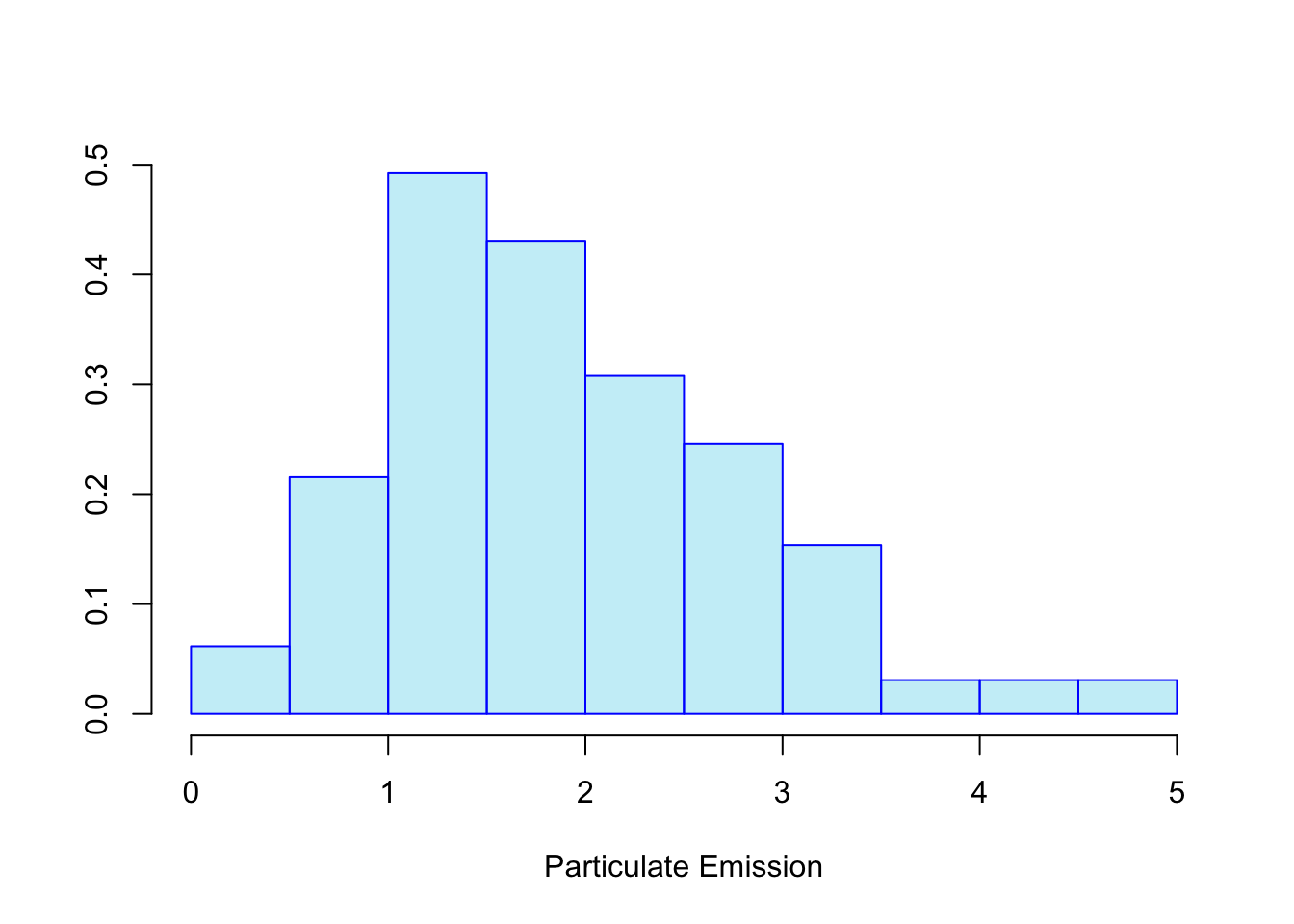
Given an experiment where a vehicle is chosed at random to have its emissions measured (grams of particles per gallon of fuel), this emission level would be a continuous value
We can place these continuous values into classes (\(0.00-0.99\), \(1.00-1.99\)) and then plot them on a histogram:
We can see how it’s possible to draw a curve across our histogram to represent the general trend of the data:
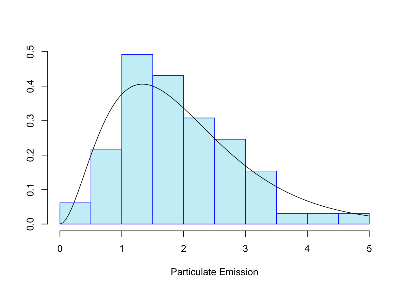
If we increase the data we collect, this histogram could get more detailed, the bars could narrow.
The more data we collect, the closer we would approach to the true distribution of the probabilities for our outcomes.
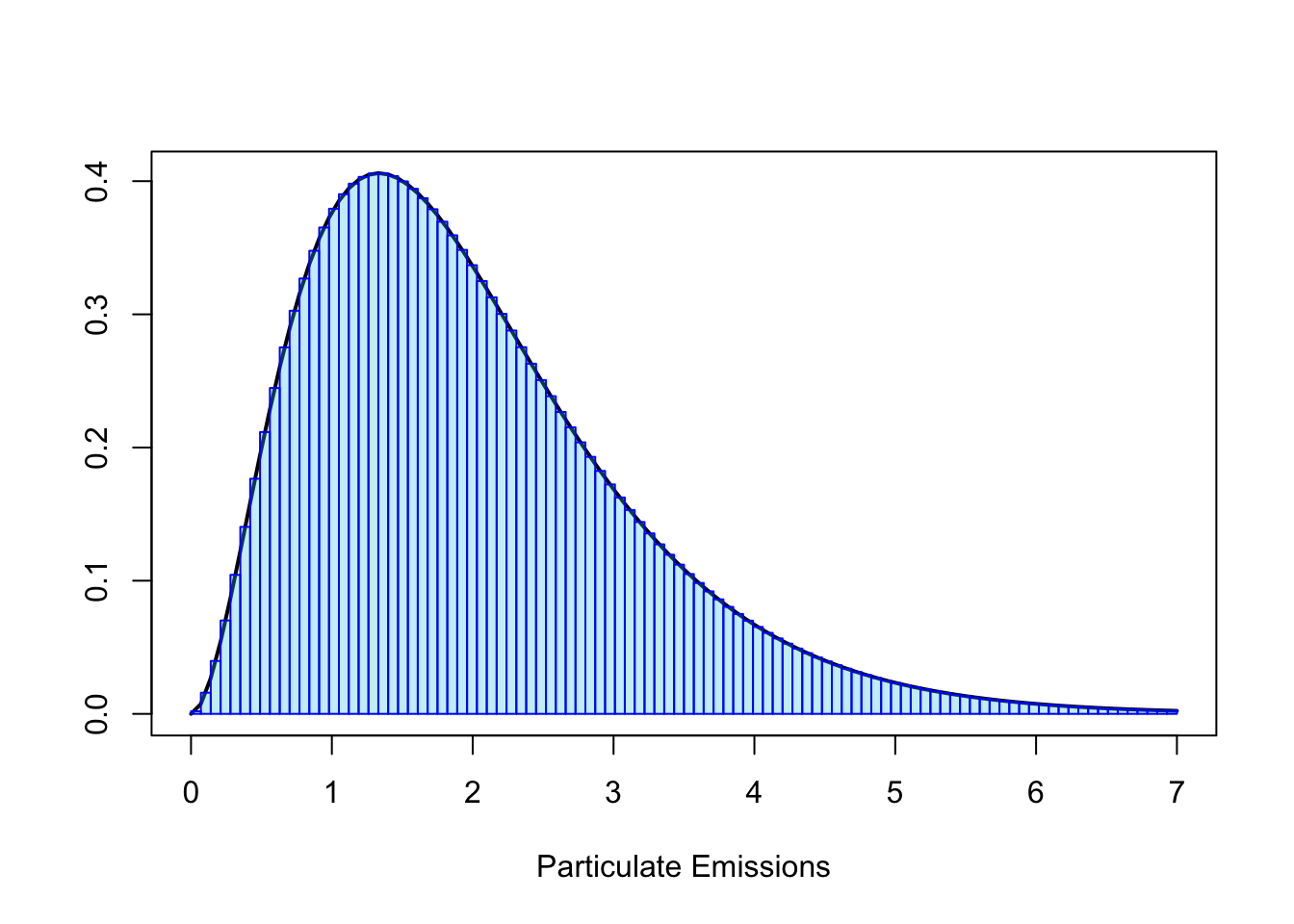
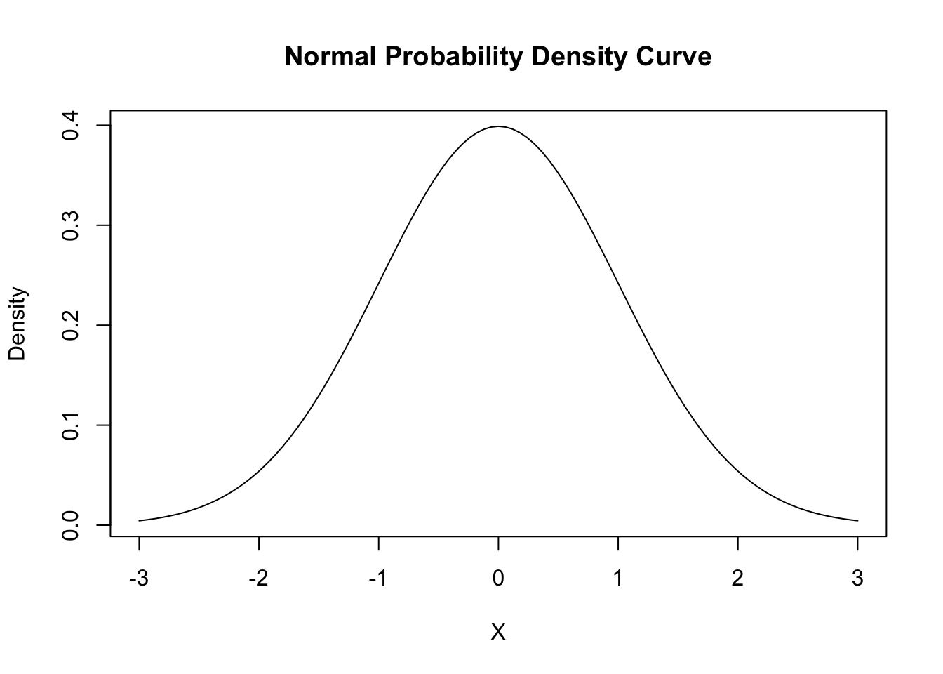
Inevitably we converge to a complete, smoothed curve:
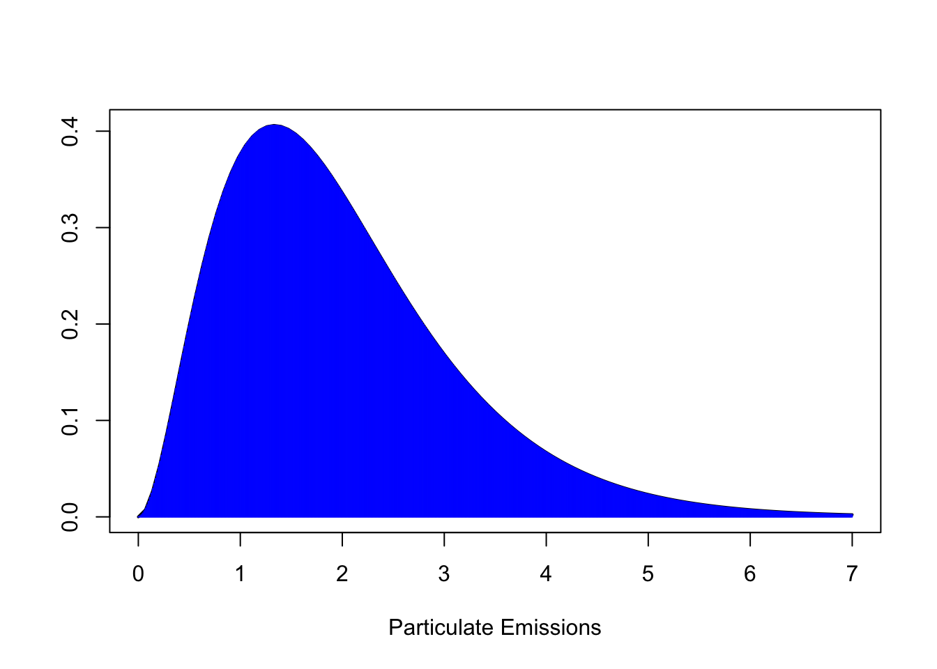
This curve is used to describe the distribution of a continuous random variable
We refer to it as a probability density curve
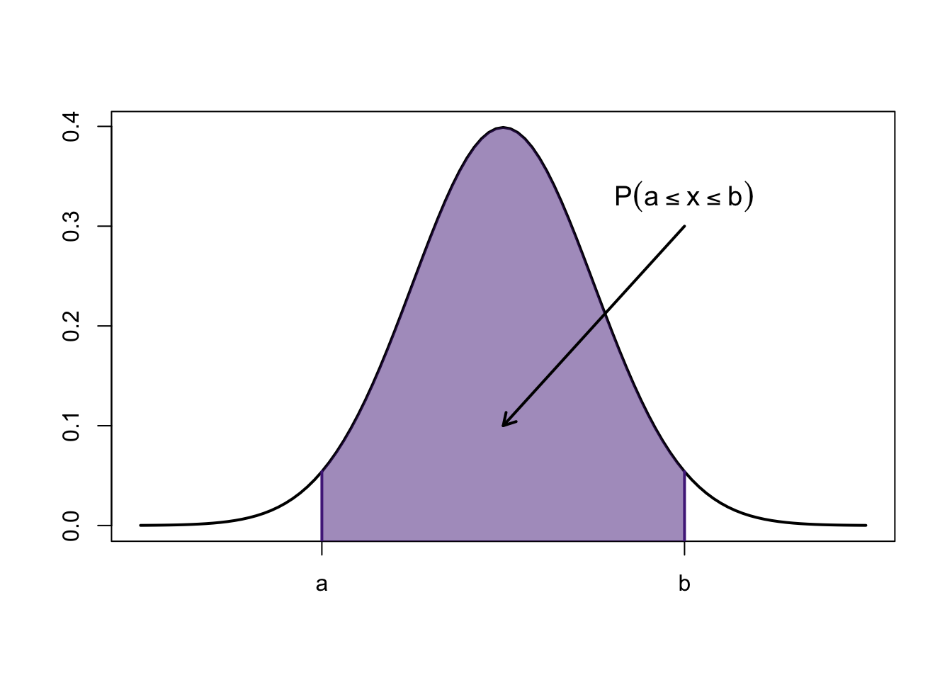
The density curve tells us what proportion of the population falls within any given interval
- Using proper language: the area under the curve between any two values \(a\) and \(b\) represents the probability that random variable \(X\) takes a value between \(a\) and \(b\)
Continuous Probability Distributions
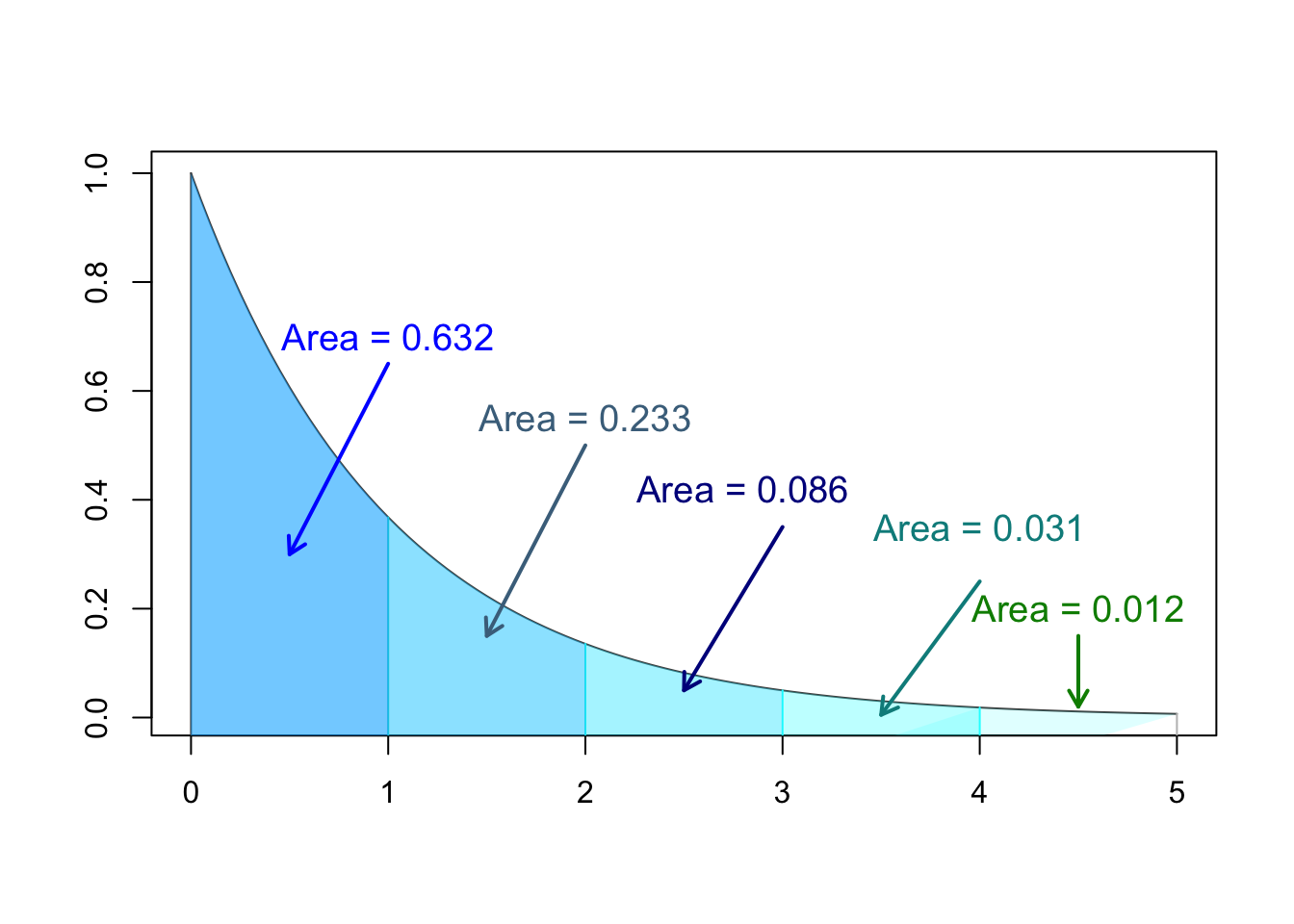
For a continuous r.v., probability is now “area under the curve”
Only intervals will have non-zero probability
- Any single value will have a probability of zero:
\[P(X=a)=0, \ \text{for any single number} \ a\]
\[P(X=b)=0, \ \text{for any single number} \ b\]
- There’s also no difference between \(\leq\) and \(<\)
\[P(X \leq 1)=P(X<1)\]
- Why is this?
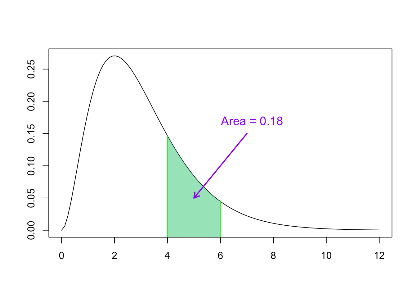
Continuous Probability Curve Example
- What is the total area of this curve?
- What is the proportion of the population between \(0\) and \(1\)?
- What is the probability of any individual in this population being between \(2\) and \(3\)?
- What is the probability of any individual in this population being between \(0\) and \(2\)?
- What is the probability of any individual in this population being greater than \(2\)?
- \(P(2 \leq x < 4)\)
- \(P(1 < x \leq 5)\)
Continuous Probability Distributions (Continued)
Probability density curves just refer to the graphical description of a continuous distribution
- This doesn’t inherently mean they’re going to be curves
If every possible value of \(X\) is equally likely then it takes on a uniform distribution
- The curve for this distribution is a horizontal bar:
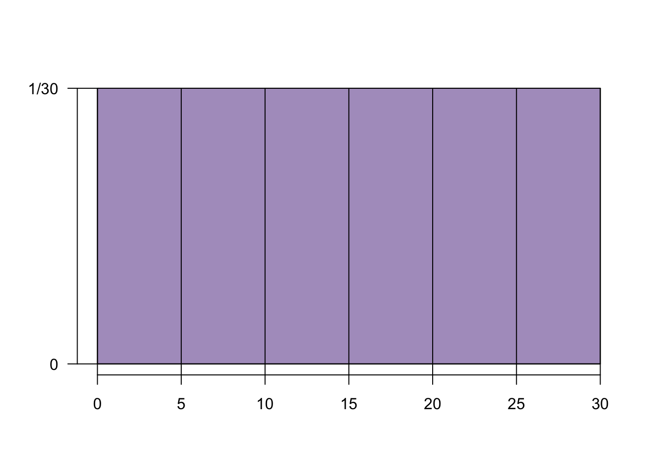
- What is \(P(5 \leq X \leq 10)\)?
- What is \(P(5 < X < 10)\)?
Word Problem
The waiting time at a bus stop for the next bus to arrive is uniformally distributed between \(0\) and \(10\) minutes.
- Find the probability that the waiting time is less than \(3\) minutes.
- Find the probability that the waiting time is greater than \(6\) minutes.
- Find the probability that the waiting time is between \(3\) and \(8\) minutes.
Continuous Distributions
The mean, variance, and standard deviation have the same interpretation for continuous variables as they do for discrete.
- To get these measurements we would need to understand calculus (or be a capable programmer)
Since neither of these are viable options for this course, we’ll instead study one of the most important examples of a continuous probability distribution: the Normal Distribution
- But not today, go away