15 Day 14
Announcements
We’re over halfway through the semester
Homework Corrections 1-8 will close 2 weeks into November
The last two corrections will close at the end of November
Stay on top of those, keep track of the due dates
Homework assignments are \(30\%\) of your grade
Why I actually do homework corrections
Review
For a continuous r.v., probability is now “area under the curve”
Only intervals will have non-zero probability
- Any single value will have a probability of zero:
\[P(X=a)=0, \ \text{for any single number} \ a\]
\[P(X=b)=0, \ \text{for any single number} \ b\]
- There’s also no difference between \(\leq\) and \(<\)
\[P(X \leq 1)=P(X<1)\]
This area, if known, can be used to make calculations on the probability of any given interval of outcomes in a continuous PDF
What is \(P(2\leq x \le 3)\)
If every possible value of \(X\) is equally likely then it takes on a uniform distribution
- The curve for this distribution is a horizontal bar:
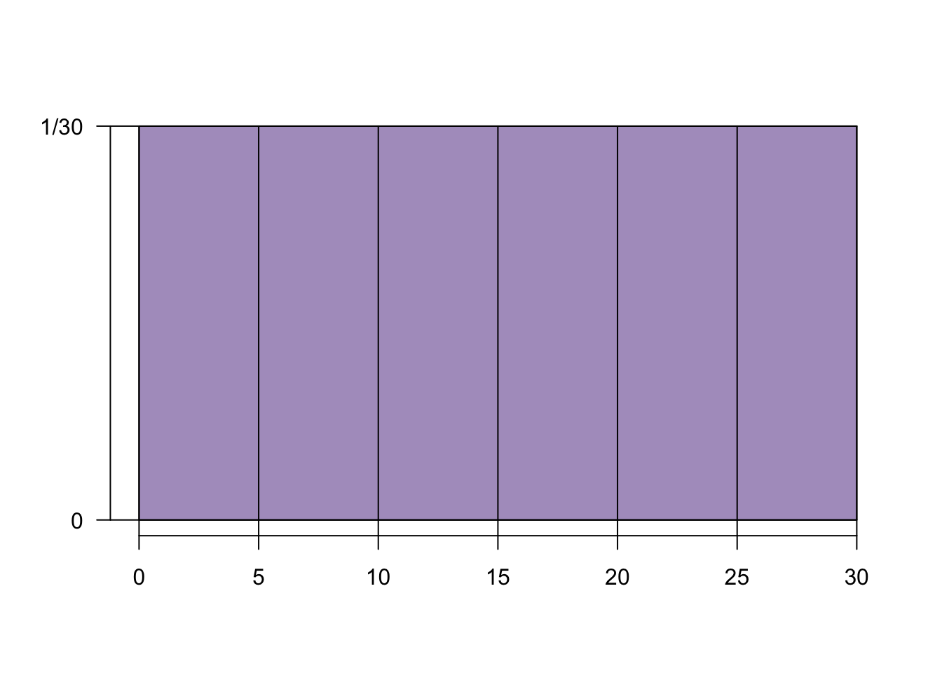
When calculating a uniform probability, consider that each value takes on that same probability:
\[\text{Given} \ P(0 < x < 5)= 5 \times{1\over 30}={5\over 30}={1\over 6}\]
\[\text{then} \ P(0 < x < 30) = 30 \times {1\over 30}={30\over 30}=1\]
\[\text{and} \ P(10 \leq x < 20) = 10 \times {1\over 30} = {10\over 30} = {1\over 3}\]
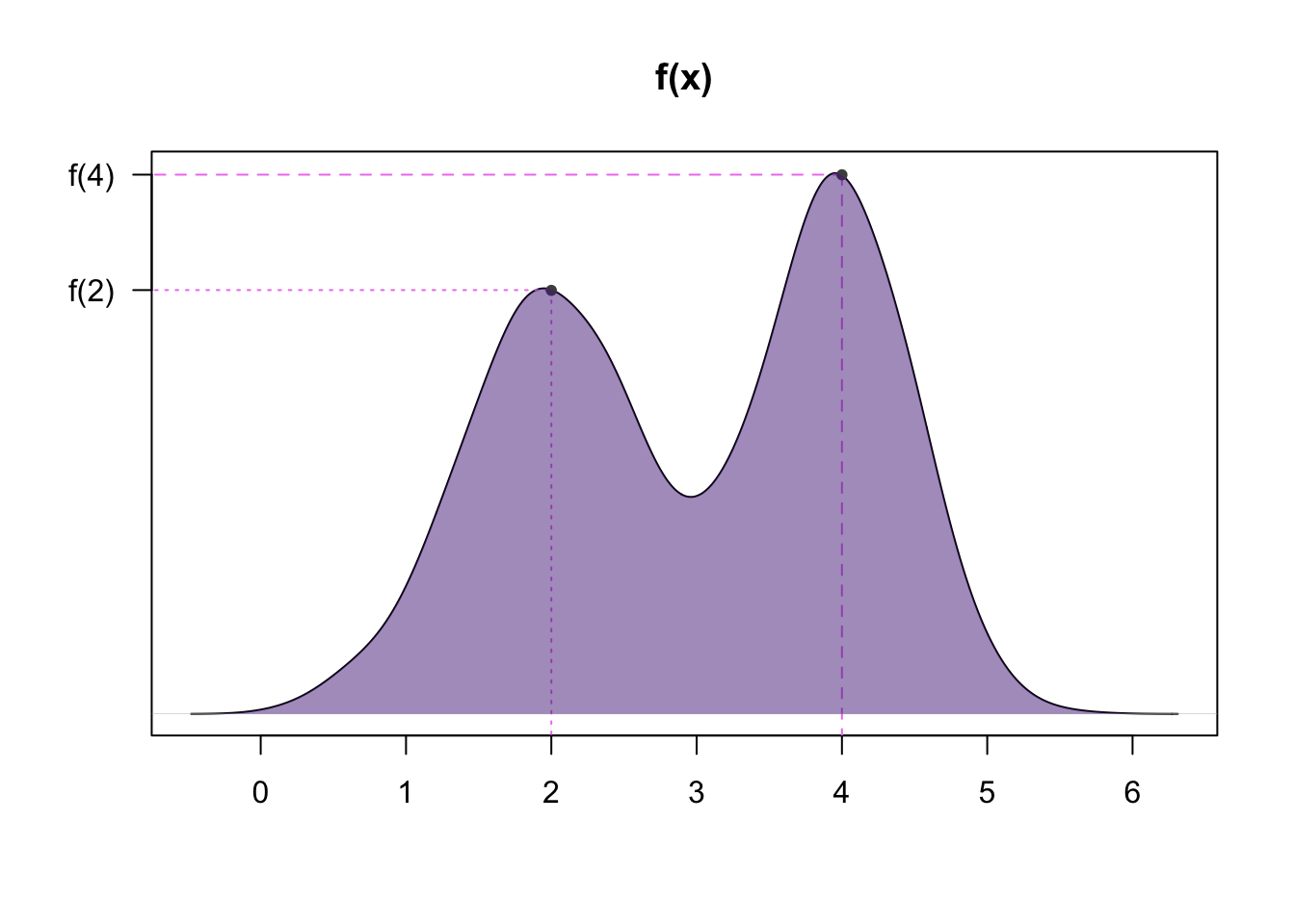
The curve used to describe the probability distribution of a continuous r.v. is called a probability density curve
- This curve is dictated by a function, \(f(x)\), called the probability density function
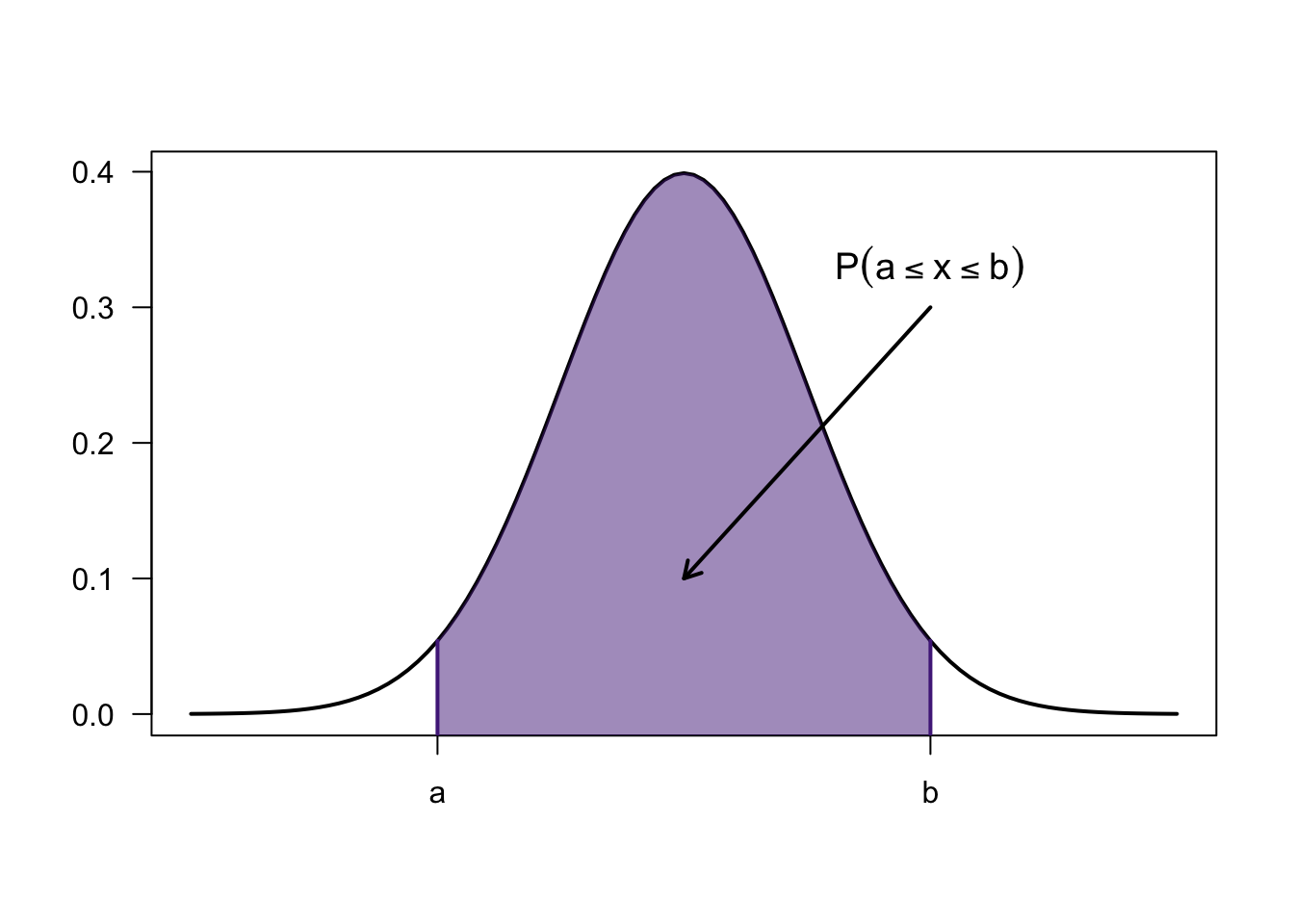
The area under the curve between two values \(a\) and \(b\) has two general interpretations:
The propotion of the population within the interval of \(a\) and \(b\) (values between \(a\) and \(b\))
The probability that a randomnly selected individual will have a value between \(a\) and \(b\) (\(P(a<x<b)\))
The area under the entire curve must equal \(1\)
- Approximated areas will rarely be a perfect value of \(1\), they just shouldn’t heavily be outside of \(1\)
Empirical Proof of Discrete Expectations
Expectation and Variance of a r.v. is a simplistic formula, but conceptually can be difficult to grasp.
In my experience “Empirical Proof”, or the results of a large scale simulation, can sometimes make these concepts easier to interpet.
The expectation of a random variable being given as:
\[\mu_x=\sum_xxP(X=x)\]
Is a theoretical simplification of an empirical study where we are somehow able to sample from our population an infinite number of times.
Given a r.v. with the following probability distribution:
\[ \begin{array}{|c|c|c|c|c|c|c|} \hline x & 0 & 1 & 2 & 3 & 4 & 5 \\ \hline P(X = x) & 0.4 & 0.2 & 0.15 & 0.1 & 0.1 & 0.05 \\ \hline \end{array} \]
We would compute \(EX\) as:
\[0(0.4)+1(0.2)+2(0.15)+3(0.1)+4(0.1)+5(0.05)=1.45\]
And \(VarX\) as:
\[=(0-1.45)^2(0.4)+(1-1.45)^2(0.2)+(2-1.45)^2(0.15)+ \newline (3-1.45)^2(0.1)+(4-1.45)^2(0.1)+(5-1.45)^2(0.05)\]
\[=2.4475\]
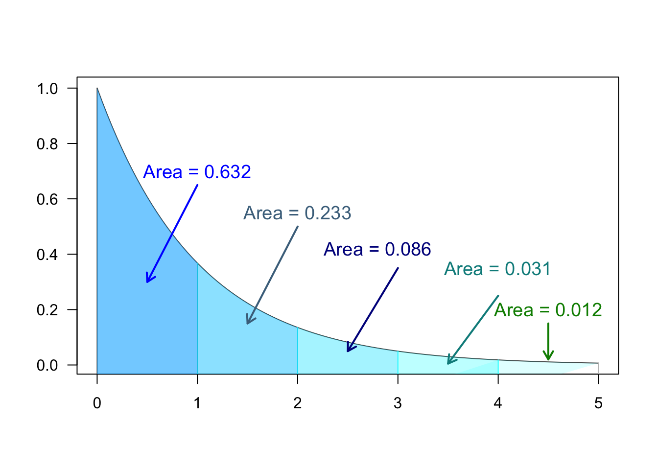
These probabilities arise from an empirical distribution of approximately infinite samples:
set.seed(1) # for reproducibility

# our values of x
x=c(0,1,2,3,4,5)

# the theoretical probabilities of x
p=c(0.4,0.2,0.15,0.1,0.1,0.05)

# 10 million samples
n=10^6

# sample our x values 10 million times
# with replacement, and their given probabilities
samp=sample(x,n,T,p)

# get the mean of our samples
mean(samp)
## [1] 1.449516## [1] 2.44431As with ALL numerical/empirical approximations, these aren’t perfect values of our theoretical calculations.
- Hypothetically, how could we make them exact to the theoretical values?
The Normal Distribution (Part 1)
The normal distribution is (un)arguably the most important probability distribution used in statistics
We’ve encountered it already in this course
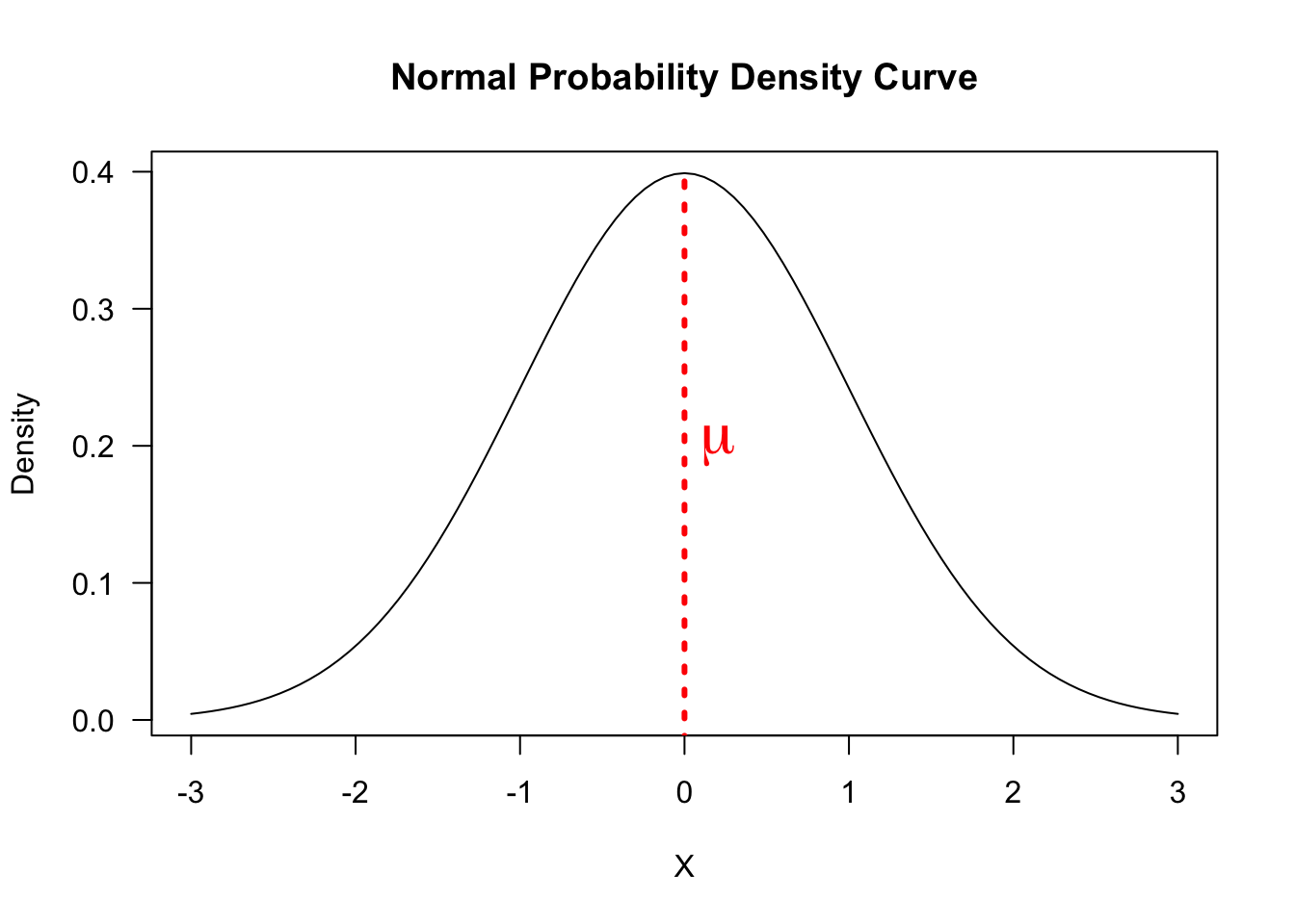
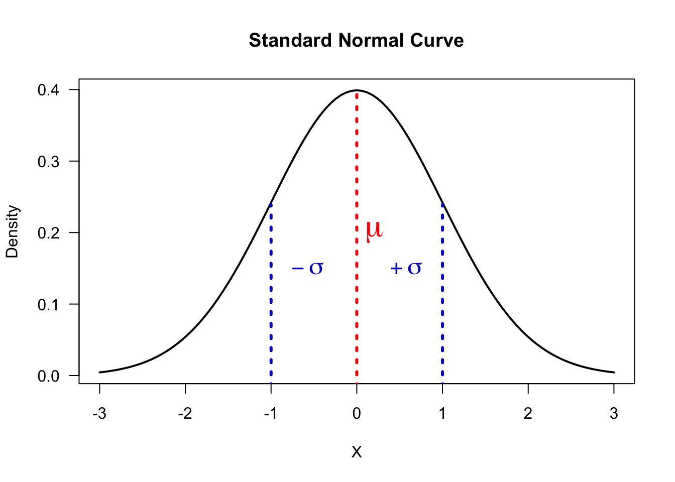
The shape of a normal distribution curve is symmetric, bell-shaped, centered around its peak
A population that is represented by a normal curve is said to be normally distributed
- or to have a normal distribution
Any normal r.v. is complete characterized by specifying values for its mean and standard deviation
The pdf for the normal distribution is given by:
\[f(x)={1\over \sigma \sqrt{2\pi}}e^{(x-\mu)^2\over 2 \sigma^2}\]
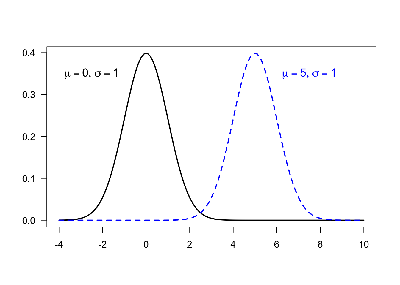
\(\mu\) is both the mean and median (due to symmetry) and is called a location parameter
- if the value of \(\mu\) is changed, the whole distribution is shifted
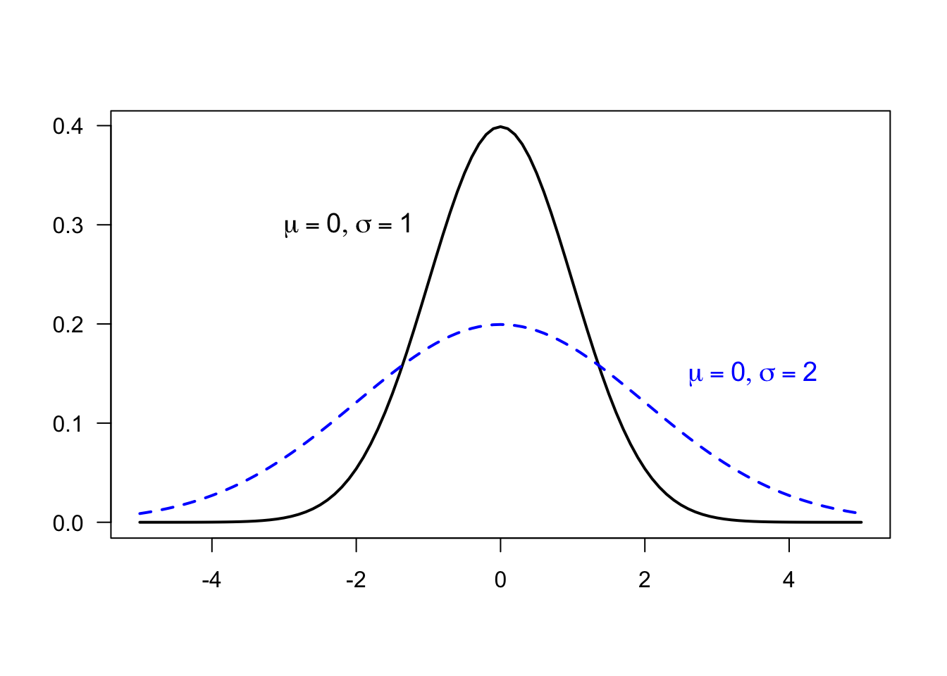
\(\sigma\) is the standard deviation and referred to as the scale parameter
- the larger \(\sigma\) is, the more “squished” the distribution looks
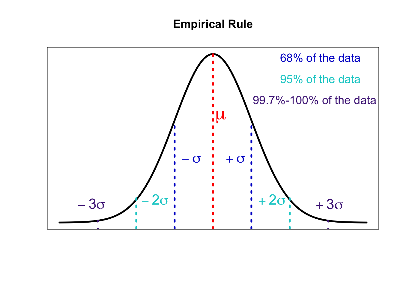
Recall a special feature of approximately bell-shaped distributions:
Standard Normal Distribution
A standard normal distribution is a normal distribution with:
\(\mu=0\)
\(\sigma = 1\)
- What is the total area under the standard normal curve?
We use the letter \(Z\) to represent a standard normal random variable (referring to \(z\)-score)
The probability that a standard normal random variable \(Z\) is between \(a\) and \(b\) (\(P(a<Z<b)\)) is equal to the area under the standard normal curve over the interval \([a,b]\)
As we’ve discussed in gruesome detail, we need calculus to manually compute this area
- Regardless of if you know calculus, for this course you do not
We’re left with some options in the absence of manual integration:
Numerical integration
Digital computation (I wish I could teach you all this)
Graphing calculators
\(z\) tables
Against my own will, my better judgement, and possibly your human rights, we will be using \(z\) tables (Table A.2 in the textbook, also posted on Canvas)
Exercise 1
Use \(Z\)-table (or Table A.2 in the textbook) to compute:
\(P (Z < 1.26)\) (i.e., area to the left of \(z = 1.26\));
\(P (Z > −0.58)\) (i.e., area to the right of \(z = −0.58\));
\(P (−0.58 < Z < 1.26)\) (i.e., area between \(z = −0.58\) and \(z = 1.26\)).
Part a
- \(P (Z < 1.26)\) (i.e., area to the left of \(z = 1.26\));
- Start by sketching an image (as a terrible artist, I’m partially going to cheat):

- Locate your value using the \(z\)-table
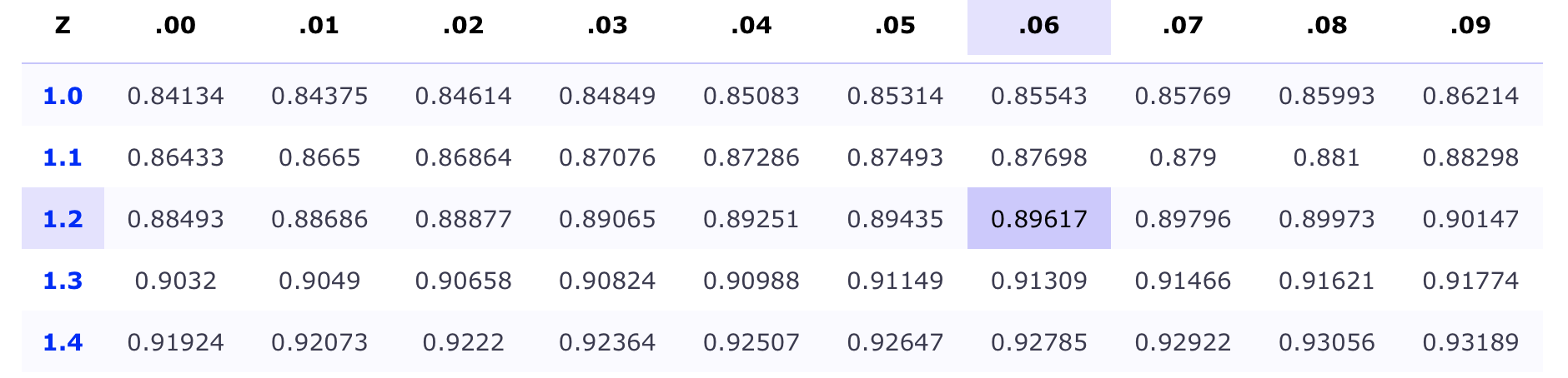
- The value \(0.8962\) is the area to the left of \(z = 1.26\)
Part b
- \(P (Z > −0.58)\) (i.e., area to the right of \(z = −0.58\));
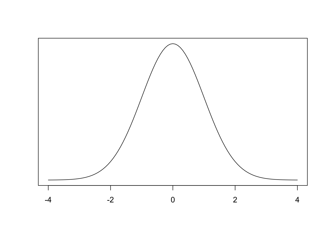
- Sketch your picture:

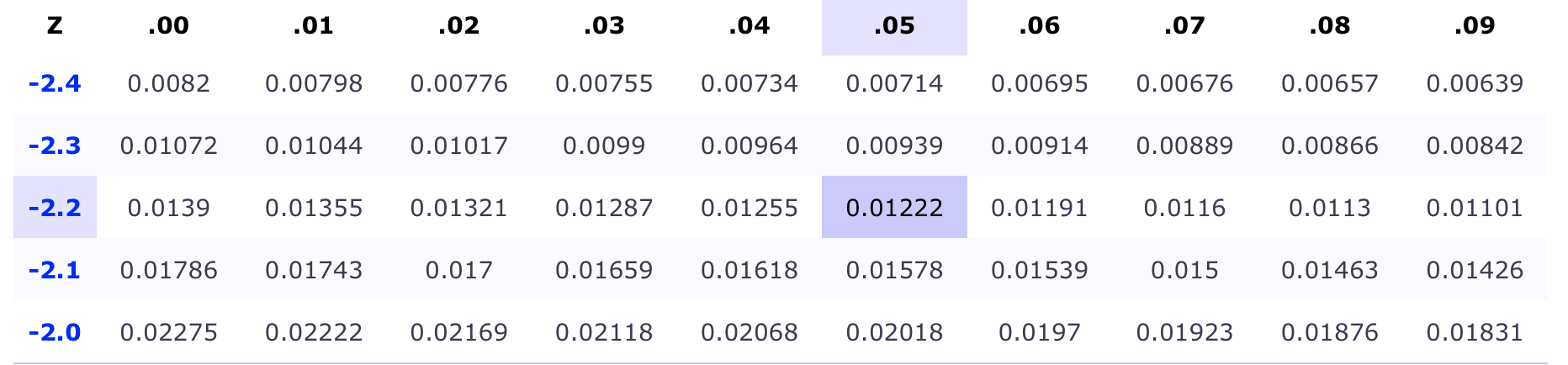
- Look up your value using the \(z\)-table
Remember that our \(z\)-table is telling use area to the left
- Use the complement rule to find the area to the right of \(z=-0.58\)
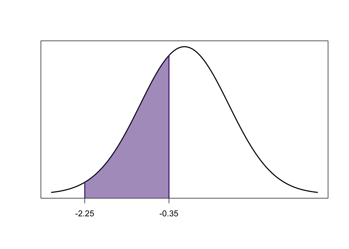
Part c
- Be an artist:
Parse the \(z\)-table if needed (we don’t need to here)
Use your results from part (a) \(P(Z < 1.26)\) and part (b) \(P(Z > −0.58)\) to compute the area between \(P(-0.58<Z<1.26)\)
Finding a z Score for a given area
Often we need to find the \(z\)-score that corresponds to a given area under the standard normal curve (e.g. percentile values).
Recall that the numbers in the body of \(z\)-table represents the area to the left of the corresponding z-score.
The next example shows how to use \(z\)-table to find the \(z\)-score given an area under the standard normal curve.
z-score Exercise 1
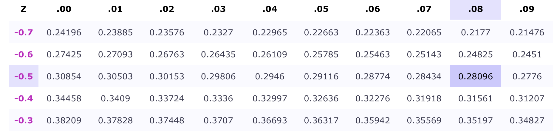
Use the \(z\)-table to find the \(z\)-score that has an area of \(0.68\) to its right.
- Sketch your curve:
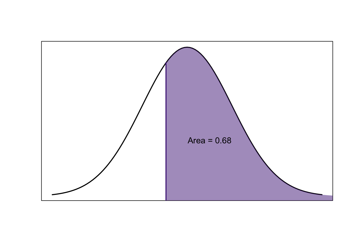
Since we want area to the left in order to use a \(z\)-table, we need to take the complement:
\[1-0.68=0.32\]
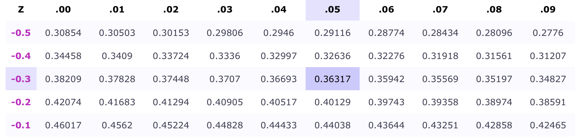
Then, recognizing that approximations will never be perfect, we’ll search our \(z\)-table for a value that’s \(\approx 0.32\):
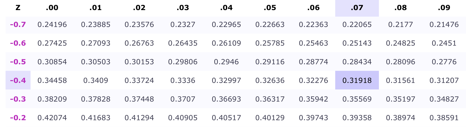
Approximations are a slight touchy feely art
We can see that \(|0.32-0.32276|=0.00276\) and \(|0.32-0.31918|=0.00082\)
It should be clear that \(0.00276>0.00082\)
So \(z=-0.47\) is a better approximation of our given area than \(z=-0.46\)
In practice you can do a lot of this determination with gut feeling and be effective
Our final conclusions is that \(z=-0.47\)

The Problem with Proving z-tables
Being told to use a system and just trust that it works may work for most of us (it definitely does for me) but some people need a deeper understanding to justify using a tool. And that’s fine!
I’ll try to give some degree of comfort that our \(z\)-table is a useful construct and not just a tool created with no basis. Additionally, I’ll (hopefully) justify that, even with several semesters of calculus education, you wouldn’t be doing any of this by hand.
Given the pdf of the normal distribution:
\[f(x)={1\over \sigma \sqrt{2\pi}}e^{(x-\mu)^2\over 2 \sigma^2}\]
Plugging in \(\mu=0\) and \(\sigma=1\):
\[f(x) = \frac{1}{\sqrt{2\pi}} e^{-\frac{x^2}{2}}\]
We can compute the definite integral of this function from \(1.96\) to \(-1.96\) to verify our \(z\)-table is valid, the issue is that this is a nasty integral to begin with:
\[\int_{-1.96}^{1.96} \frac{1}{\sqrt{2\pi}} e^{-\frac{x^2}{2}}\ dx\]
It ends up resolving to an equation involving the Gaussian Error Function:
\[={1\over 2}\left[1+ erf(x)\right]\]
Where we’d plug in our upper and lower bounds of the definite integral to complete the computation.
Being able to complete this computation to the point we get to that error function is a process at a high enough caliber we’d legitimately need to push through several high level calculus courses to explain the necessary steps.
However, numerical integration let’s us make this slightly more intuitive.
While far from the most accurate or efficient method of calculating the area under a curve numerically, the trapezoidal rule allows us to cut up the curve into small trapezoids and compute their area to avoid performing a nasty amount of analytical calculus.
Cutting up hypothetical pieces of paper and measuring them is a lot more intuitive than \(u\)-substitution, partial integration, and known form integral usage:
# standard normal pdf
f=Vectorize(function(x) {
  return((1/sqrt(2*pi))*exp(-x^2/2))
})

# trapezoidal rule
trapez=function(f,a,b,n) {
   # trapezoid width
  h=(b-a)/n
  x=seq(a,b,length.out=n+1)
  y=f(x)
  inte=(h/2)*(y[1]+2*sum(y[2:n])+y[n + 1])
  return(inte)
}

# lower bound
a=-1.96
# upper bound
b=1.96
# number of trapezoids
n=10000

area=trapez(f,a,b,n)
1-area
## [1] 0.9545329