5 Day 4
Announcements:
-
One of the other instructors made this
Thanks Eli!
No office hours today
Thursday 9 AM - 10 AM
After 2:45 PM please do not talk to me
Stat Help Lab
- Should open next week
Homework point recovery will open after this class
No due date but please respect my time
- Don’t give me 10 homeworks on November \(1^{st}\)
I’m not going to grade them yet
- Don’t stress email me, I won’t reply
Extracurricular questions and supplemental material
Review
- When we have one quantitative variable we have several options:
Histograms
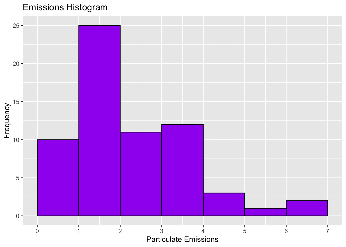
Histogram: visual representation of a frequency distribution
- Not a bar graph
Start by making a frequency distribution:
Define classes (numeric intervals)
Record the frequency of occurrences
| Class | Frequency |
|---|---|
| 0.00-0.99 | 9 |
| 1.00-1.99 | 26 |
| 2.00-2.99 | 11 |
| 3.00-3.99 | 13 |
| 4.00-4.99 | 3 |
| 5.00-5.99 | 1 |
| 6.00-6.99 | 2 |
Lower class limit: the smallest value that can appear in that class
Upper class limit: largest value that can appear in that class
Class width: the difference between consecutive lower class limits
General requirements for quantitative frequency distributions:
Every observation must fall into one of the classes
The classes must not overlap
The classes must be of equal width
There must be no gaps between classes
Bar height (y-axis) represents class frequency
Bar width (x-axis) represents class width
Left edge of each bar corresponds to the lower class limit
No gaps between classes so no gaps between bars of a histogram
We care about the shape of our data
The shape of our data can help us observe the distribution of our data
Vocabulary for describing the shape of data:
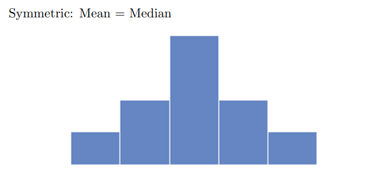
Symmetric - mirror image on both sides of it’s center
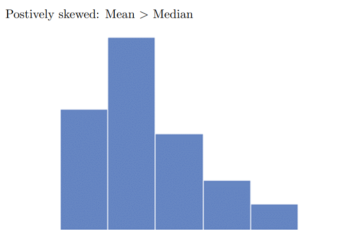
Positively-skewed - Long, narrow tail to the right
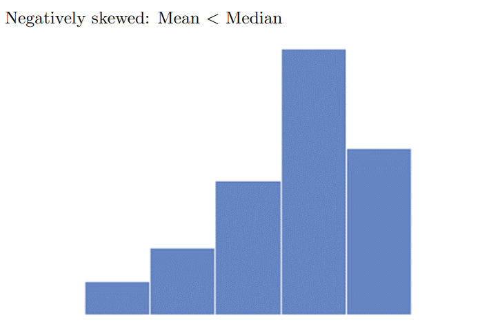
Negatively-skewed - Long, narrow tail to the left
Unimodal - One peak/hump
Bimodal - two peaks/humps
Uniform - b o x
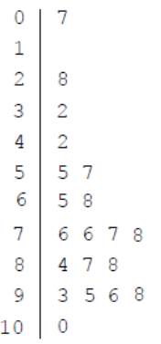
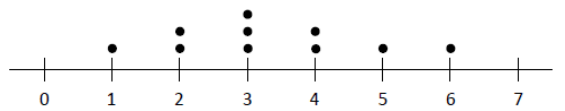
Histograms can be used to summarize both small and large data sets
Sometimes we prefer more detailed visualizations for smaller data sets

Numerical Descriptions
Graphics are good for taking data and making it easier to view
Numerical summaries are how we take data and make it easier to understand
We’re going to specifically cover:
Mean
Median
Mode
Refresher:
A parameter describes a population
A statistic describes a sample
“Use of sample statistics to describe population parameters”
- Statistical Inference in a nutshell
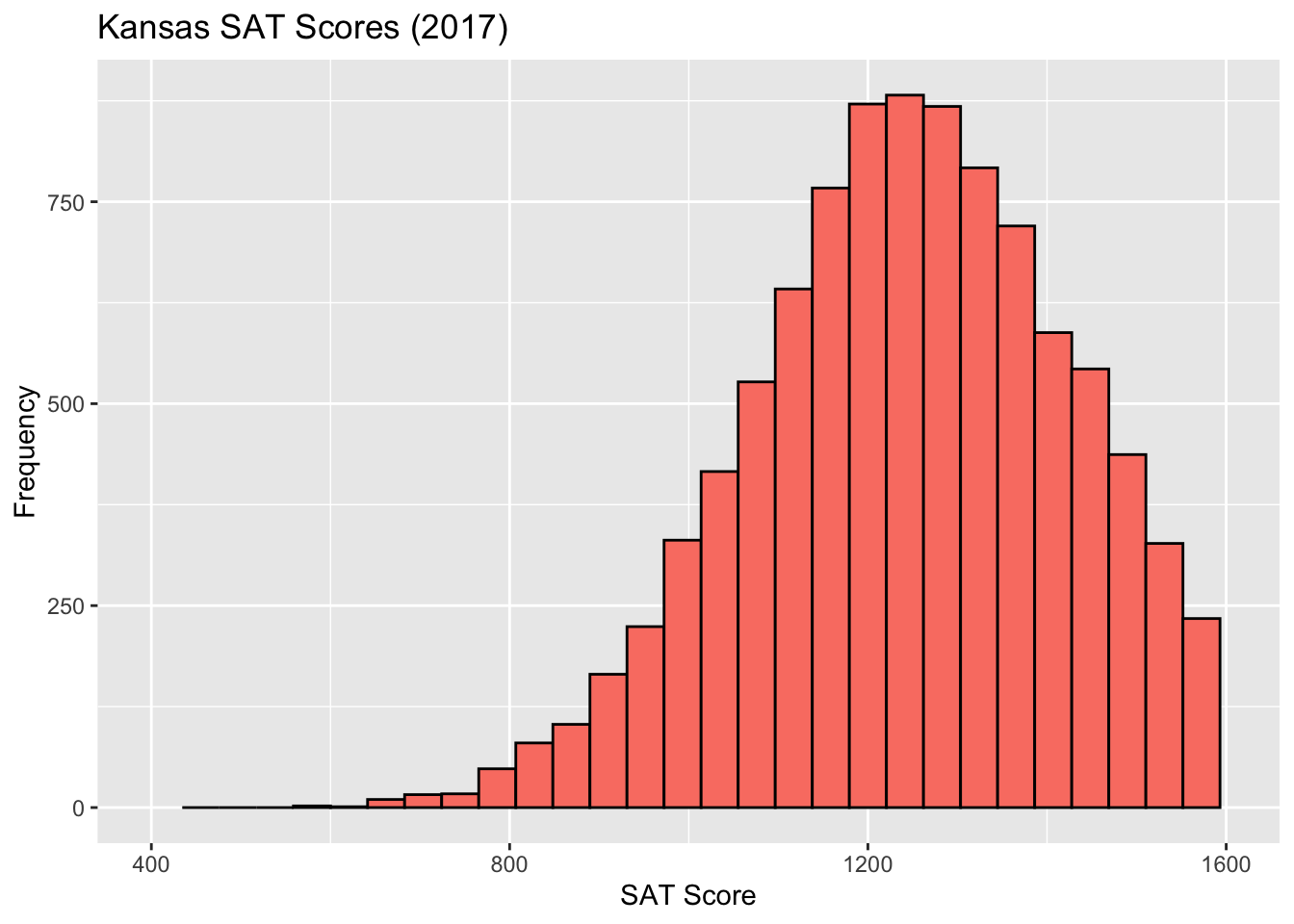
Which way is this histogram skewed?
How would you describe the “center” of this data?
Mean or average: Balance point (fulcrum) of the dataset.
Median: Half of the data points are above the median, half are below.
Mode: Where the peak is.
Mean
Most commonly used metric for summarizing data
Sum all of the data then divide by the number of observations
| 7 | 3 | 12 | 3 | 5 |
\[Mean \ = \ {7+3+12+3+5 \over 5} = {30 \over 5} = 6\] - If the data we calculated a mean for comes from a sample:
Sample mean
If the data we calculated a mean for comes from a population:
- Population mean
Which one is a parameter?
- A statistic?
Mathematical Notation Soapbox
“Letter math”
I resisted it forever
But trust me, it does end up being helpful
Data values can be denoted as \(x_1,x_2,x_3,...\)
\(x_1\) refers to the observed value of the variable \(x\) from individual 1
\(x\) can be anything
It doesn’t even have to be \(x\)
It’s convention, not law
Sample size (the number of individuals in the sample)
- Denoted with \(n\) (Note: lower-case)
Population size
- Denoted with \(N\) (Note: capital)
Summation:
This is referring to the sum (addition) of everything contained in the expression
We denote this with the Greek letter \(\Sigma\)
With this notation we can describe:
\[\sum\limits_{i=1}^nx_i=x_1+x_2+...+x_n\]
“The summation of \(x_i\) to the \(n^{th}\) term, indexed by 1”
With sigma notation we can express the sample and population mean formulas:
- Sample mean (denoted \(\bar{x}\)):
\[{1 \over n}\sum\limits_{i=1}^nx_i\]
- Population mean (denoted \(\mu\)):
\[{1 \over N}\sum\limits_{i=1}^Nx_i\]
Greek letters usually mean population parameters
Lower-case letters usually mean sample statistics
In practice:
| Student | Absences |
|---|---|
| 1 | 2 |
| 2 | 6 |
| 3 | 1 |
| 4 | 2 |
| 5 | 4 |
| 6 | 0 |
| 7 | 1 |
| 8 | 3 |
| 9 | 0 |
| 10 | 2 |
\[{1 \over n}\sum\limits_{i=1}^nx_i\] \[{1 \over 10}(x_1+x_2+x_3+x_4+x_5+x_6+x_7+x_8+x_9+x_{10})\]
\[{1 \over 10}(2+6+1+2+4+0+1+3+0+2)\]
\[{1 \over 10} *21 = {21 \over 10} = 2.1\] - Properties of mean:
Common
Easy to interpret
Susceptible to outliers
The average number of Super Bowl rings between me and Tom Brady is 3.5
(As of 2021) the top 1% of households in the United States hold 32.3% of the country’s wealth, while the bottom 50% hold 2.6%
A statistic is resistant if its value is not affected heavily by outliers
- Is the mean resistant?
Median
- Middle value, half the data are below and half are above
| 7 | 3 | 12 | 3 | 5 |
- Sort your data in increasing order (low to high)
| 3 | 3 | 5 | 7 | 12 |
The median is 5
If \(n\) is odd: choose position \({(n+1)\over2}\) in the ordered dataset
So \(n=5\)
\[{(n+1)\over2}={(5+1)\over2}=3\]
- We pick the \(3^{rd}\) data point after sorting
| 7 | 3 | 12 | 3 | 5 | 8 |
If \(n\) is even after ordering:
Pick \(n\over 2\) and \({n \over 2}+1\)
Average the two data points
| 3 | 3 | 5 | 7 | 8 | 12 |
So \(n=6\)
\[{6\over 2}=3 \ ,\ {6 \over 2}+1=4\]
3rd data point: \(5\)
4th data point: \(7\)
\[{(5+7)\over 2}=6\]
- The median is \(6\)
Properties of median:
It doesn’t use all of the data directly
This makes it resistant
- Outliers have little/no effect
Sometimes a more realistic measurement:
Median Household Income (Kansas): \(\$57,422\)
Average Household Income (Kansas): \(\$77,509\)
Why does median make more sense than average here?
Difference between median and mean depend on skew of the histogram
Mode
The most frequent observation
Useful for qualitative data
- “Which credit card is most commonly used by our customers?”
Not as useful for quantitative data
“What’s the most common weight of cattle on our research farms?”
Why isn’t this a helpful metric?
A data set can have any number of modes (0,1,2,…)
| 7 | 3 | 12 | 3 | 5 |
The most frequently observed value in this data set is \(3\)
- So the mode is \(3\)
The below data set displays a sample of \(n=7\) observations:
| 2 | 1 | 3 | 4 | 3 | 5 | 4 |
Find the mean, round to two decimal places if necessary:
Find the median, round to two decimal places if necessary:
Find the mode(s):
A group of restaurants reported in a recent year that the mean price for their dinner was \(\$18\), and the median was \(\$22\). If a histogram was constructed for the price of dinner at the group of restaurants, would you expect it to be skewed to the right, skewed to the left, or approximately symmetric?