19 Day 18

Announcements

• Exam next week

• Study now, make this the easy exam

  • Review session Wednesday

  • Come with questions on the content of the exam

  • We’ll be reviewing different content that a few instructors have made

  • Cheat sheet design session as well

• Day 19 content is partially shoved into Today’s lecture

  • That’s why we can do review on Wednesday

Review

Uncertainty and Statistics

“All models are wrong, but some are useful” - George E. P. Box

What is the primary goal of statistics?

• Can we achieve this goal without making any errors?

We define uncertainty from two central concepts:

• For every population we can draw information from, there is a sample $X$

  • The mean of our sample is $\bar{x}$

  • $\bar{x}$ is assumed to be normally distributed under two circumstances

    • 1. The distribution of $X$, and thus our population, is NORMAL
    • 2. Our sample size of $X$ is $>30$

Why does point (1) make sense?

• If we draw samples from a population that has any distribution

  • It’s samples will have the same distribution

  • A condition where this doesn’t hold is when we transform our data somehow

    • i.e., Taking samples from a normally distributed population but transforming the samples to strictly positive, discrete values

Why does point (2) make sense?

• In applied statistics we check our assumptions

  • Logically the only way to check this assumption would be to take a lot of samples

  • We’ve done that outside of this class, our assumptions do hold (refer to the CLT App in the bookdown)

• Logically however:

  • We assume that the distribution of $\bar{x}$ is normal even upon one observation arising from a sample of $n>30$

  • Empirical and mathematical proof are shockingly easy to obtain (and do by hand!)

  • I do recommend just seeking out a program to do it for you however

When we sample from a population, and compute a statitic, we’re always slightly wrong

• Statistics accepts errors on the single condition that you can quantify those errors

Central Limit Theorem

Given we have an understanding of the CLT, most of this class should feel essentially intuitive

The Central Limit Theorem boils down to the statement that:

• “…a large, properly draw sample will resemble the population from which it is drawn.” - Charles Wheelan

Think about sampling $40$ defensive linemen from random college football teams

• We can pretty intuitively assume that they’re going to be pretty heavy on average

• If we got an average weight of $140$ lbs. we’d be concerned we sampled wrong

  • Not because it’s impossible

  • But because it’s highly unlikely

That’s it.

Confidence Intervals are a way to quantify uncertainty

• Put simply, we’re saying “The true value is $X$, give or take $a$”

We have two methods for calculating confidence intervals:

1. $z$-method (given $\sigma$ is known)

$$\bar{x} \pm z_{\alpha/2} \cdot \frac{\sigma}{\sqrt{n}}$$

2. $t$-method (given $\sigma$ is unknown)

$$\bar{x} \pm t_{\alpha/2} \cdot \frac{s}{\sqrt{n}}$$

$t$-method refers directly to the Students t-distribution

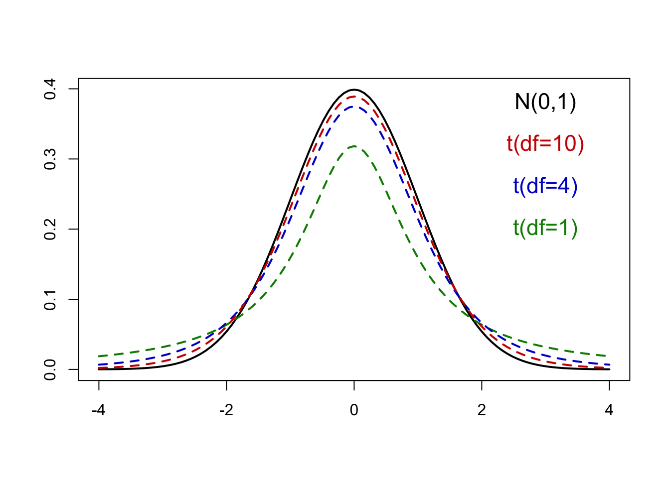
• Similar to the standard normal distribution

  • Unimodal

  • Symmetric around $0$

• Wider (or heavier) tails than the standard normal

  • Meaning it’s more spread out

• Distinguished by degrees of freedom ($df = n - 1$)

  • As $df$ increase the t-distribution converges to a normal distribution

In practice, we always use the t-method

• Why?

Confidence Intervals for Proportions

• To get a confidence interval we need:

  • Point estimate

  • Margin of Error

• Our point estimate for $p$ (population proportion):

  • $\hat{p}$

• Margin of error is given by:

$$z_{\alpha/2} \sqrt{\frac{\hat{p}(1 - \hat{p})}{n}}$$

• We need to justify being able to make a confidence interval

• Given the CLT for proportions:

$$n\hat{p} \geq 10 \quad \text{and} \quad n(1 - \hat{p}) \geq 10$$

then the $100(1 - \alpha)\%$ confidence interval for $p$ is:

$$\hat{p} \pm z_{\alpha/2} \sqrt{\frac{\hat{p}(1 - \hat{p})}{n}} \quad \text{(Margin of Error)}$$

• Recall that the critical value $z_{\alpha/2}$ comes from the standard normal distribution.

Example 1: Sleep Apnea

Sleep apnea is a disorder in which there are pauses in breathing during sleep. In a sample of 427 people aged 65 or over, 104 had sleep apnea.

a. Find a point estimate for the population proportion of those aged 65 and over who have sleep apnea. (Round your answer to 3 decimal places.)

$$\hat{p} = \frac{104}{427} \approx 0.244$$

b. Compute the margin of error for a 99% confidence level.

For 99% confidence, $\alpha/2 = 0.005 \Rightarrow z_{\alpha/2} = 2.576$. The margin of error is:

$$z_{\alpha/2} \times \sqrt{\frac{\hat{p}(1 - \hat{p})}{n}} = 2.576 \times \sqrt{\frac{0.244(1 - 0.244)}{427}} \approx 0.054$$

c. Construct a 99% confidence interval for the proportion of those aged 65 or over who have sleep apnea.

We construct the 99% confidence interval for $p$ by:

$$\hat{p} \pm \text{Margin of Error} \Rightarrow 0.244 \pm 0.054$$

or $(0.190, 0.298)$

d. Does it appear that more than 9% of elderly people have sleep apnea? Yes, all the values in the CI are greater than 0.09.

Example 2: Sleep Study

Researchers want to estimate the mean amount of sleep per night for students at Upper Midwest University. A sample of 15 students had an average of 6.4 hours per night and a standard deviation of 1.27 hours.

a. Should we use the z-method or t-method?

$t$ method, because $\sigma$ is unknown.

b. Find a point estimate for the mean amount of sleep per night for UMU students.

$$\bar{x} = 6.4$$

c. Compute the margin of error for a 90% confidence level. (Round your answer to 3 decimal places.)

$$\alpha = 1 - 0.90 = 0.10 \Rightarrow \alpha/2 = 0.05$$

With $df = n - 1 = 14$, $t_{\alpha/2} = 1.761$ from the t-table. Compute the margin of error:

$$t_{\alpha/2} \times \frac{s}{\sqrt{n}} = 1.761 \times \frac{1.27}{\sqrt{15}} \approx 0.577$$

d. Construct a 90% confidence interval for the mean amount of sleep per night for students at UMU.

The 90% CI for the mean amount of sleep is:

$$\bar{x} \pm \text{Margin of Error} \Rightarrow 6.4 \pm 0.577$$

or $(5.823, 6.977)$

e. Does the confidence interval contradict a claim that the mean amount of sleep for UMU students is 6 hours? Explain.

No, because 6 is contained in the confidence interval.

Example 3: SAT Scores

A college admissions officer sampled 107 freshmen and found that 38 scored more than 510 on the math SAT.

a. Find a point estimate for the proportion of all entering freshmen at this college who scored more than 510 on the math SAT. (Round the answer to 3 decimal places.)

$$\hat{p} = \frac{38}{107} \approx 0.355$$

b. Compute the margin of error for a 95% confidence level. (Round your answer to 3 decimal places.)

$$\alpha = 1 - 0.95 = 0.05 \Rightarrow \alpha/2 = 0.025 \Rightarrow z_{\alpha/2} = 1.96$$

Compute the margin of error:

$$z_{\alpha/2} \times \sqrt{\frac{\hat{p}(1 - \hat{p})}{n}} = 1.96 \times \sqrt{\frac{0.355(1 - 0.355)}{107}} \approx 0.091$$

c. Construct a 95% confidence interval for the proportion of all entering freshmen who scored more than 510 on the math SAT.

$$\hat{p} \pm \text{Margin of Error} \Rightarrow 0.355 \pm 0.091$$

or $(0.264, 0.446)$.

We are 95% confident that between 26.4% and 44.6% of the entering freshmen scored more than 510 on the math SAT.

Hypothesis Testing

My philosophy for scientific communication should be apparent by now:

• Why should you care?

• What does this do?

• Why do we use this?

• Making claims about statements is how science works

  • We can convert statements into parameters, and make claims about them using statistics

• We call this: “Hypothesis Testing”

• In hypothesis testing, there are two competing statements about population parameters:

$$H_0\equiv \text{null hypothesis} \quad \text{vs} \quad H_1 \equiv \text{alternate hypothesis}$$

Upon forming these statements:

• We use data collected from a sample to test if we

  • Reject $H_0$, thereby supporting $H_1$

• A statistical hypothesis is often a statement about population parameter(s)

• The null hypothesis, $H_0$, states that the parameter is equal to a specific value

$$H_0 : \mu = 35$$

• The alternate hypothesis, $H_1$, states that the value of the parameter differs from the value specified by the null hypothesis

  $$H_1 : \mu < 35$$

  $$H_1 : \mu > 35$$

  $$H_1 : \mu \neq 35$$

• There are three types of alternate hypothesis

  • Consider $H_0 : \mu = 35$

1. $H_1 : \mu < 35$ $\Rightarrow$ called left-tailed alternate hypothesis

2. $H_1 : \mu > 35$ $\Rightarrow$ called right-tailed alternate hypothesis

3. $H_1 : \mu \neq 35$ $\Rightarrow$ called two-tailed alternate hypothesis

• Left-tailed and right-tailed hypotheses are called one-tailed hypotheses

• A null hypothesis is generally thought of as a default state of nature (e.g. existing knowledge)

• An alternate hypothesis, on the other hand, contradicts the default state (e.g. new knowledge)

• In most cases, whatever we wish to establish is placed in the alternate hypothesis

• After developing $H_0$ and $H_1$, we collect a set of data

• Based on the data, we construct a test statistic to reach one of the following decisions:

  • Reject $H_0$

  • Fail to reject $H_0$

• If we reject $H_0$

  • We conclude that $H_1$ is true

• If we fail to reject $H_0$

  • We conclude that the data do not provide enough evidence to reject $H_0$

Errors in Hypothesis Testing

• We’re making inference from samples

  • We will be a certain amount of wrong

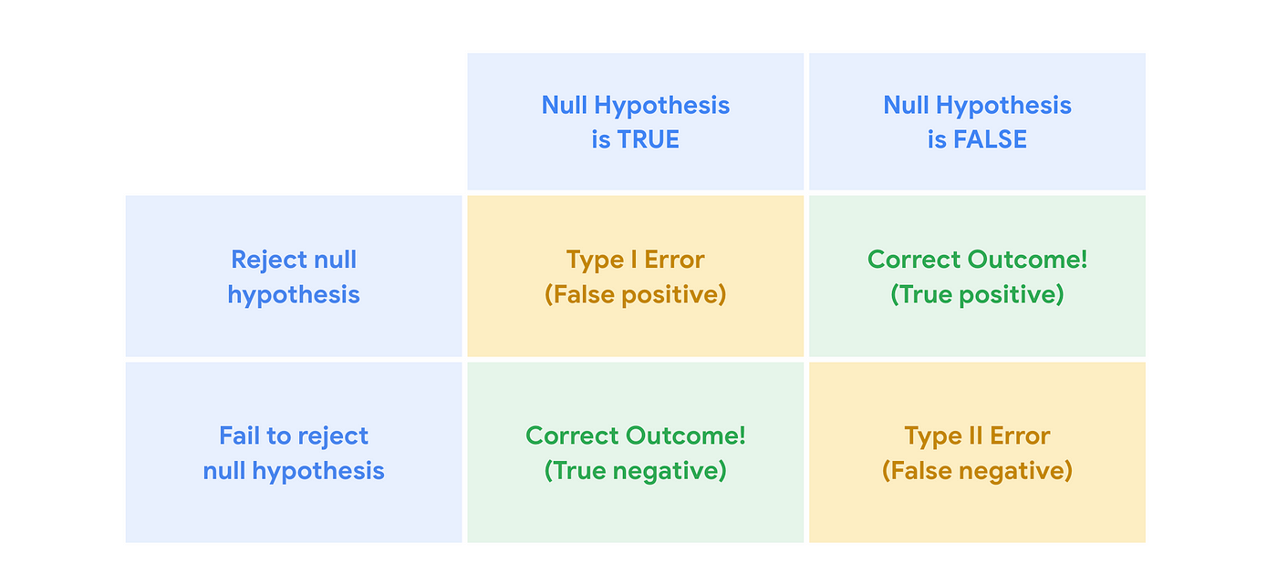
  • Depending on how wrong we are, and in what way, we define two types of errors

• Type I error: $H_0$ is true in reality, but we reject $H_0$

• Type II error: $H_1$ is true in reality, but we do not reject $H_0$

$$\begin{array}{|c|c|c|} \hline \text{Decision} & H_0 \ \text{True} & H_0 \ \text{False} \\ \hline \text{Reject} \ H_0 & \text{Type I error} & \text{Correct decision} \\ \hline \text{Don’t reject} \ H_0 & \text{Correct decision} & \text{Type II error} \\ \hline \end{array}$$

• The probability of having the Type I error is denoted by $\alpha$

• The probability of having the Type II error is denoted by $\beta$

• Minimizing both $\alpha$ and $\beta$ is impossible due to a trade-off between $\alpha$ and $\beta$

  • If we decrease $\alpha$, then $\beta$ tends to increase

• In general, controlling $\alpha$-level (chance of making Type I error) is more important since Type I error leads to the acceptance of incorrect new knowledge

• Go away