Chapter 16 複線性迴歸分析
16.1 續,劍指「成本函數」
我們在第五章已經知道最小平方法(LS)的
「適當的」
是這個意思
\[\min_{\beta_0, \beta_1} \sum (y - \hat y)^2 = \sum (y - (\beta_0 + \beta_1 \times x))^2\]
接下來,我們,雖然不是作者小編「想要的、想到的、經驗的」,我們想要把前述的
「適當的」
換成
\[\min_{\beta_0, \beta_1} \sum (y - (\beta_0 + \beta_1 \times x))^2 + \lambda (\beta_0^2 + \beta_1^2)\]
或是改成
\[\min_{\beta_0, \beta_1} \sum (y - (\beta_0 + \beta_1 \times x))^2 + \lambda (|\beta_0| + |\beta_1|)\]
接下來,這一章似乎只有一條路可以走
非常數學!!!
其實不然,作者小編依舊
想用、享用R程式碼示範各種想法並回答各式各樣的問題。
所以,接下來還是請讀者諸君不要轉台,繼續欣賞R可以變出甚麼圖像、意象、花樣來?
…
16.2 續,劍指「走過提升解釋能力之路」
Ridge and LASSO regression are some of the simple techniques to reduce model complexity and prevent over-fitting which may result from simple linear regression.
16.4 準備工作
16.4.1 波士頓數據集
require(MASS) # 用「require」不用「library」,是因為如果R已經將套件MASS載入環境,就不需要再載一次。
data(Boston)
boston <- Boston
# 「不動」原始數據集,不論它有「多原始」,是R程式設計的一項絕佳習慣。
# 即便一般使用者是無法任意改變套件MASS的內容物!
### rad (index of accessibility to radial highways)
boston[,"rad"] <- factor(boston[,"rad"], ordered = TRUE)
### chas (= 1 if tract bounds river; 0 otherwise)
boston[,"chas"] <- factor(boston[,"chas"])
head(boston)
## crim zn indus chas nox rm age dis rad tax ptratio black lstat
## 1 0.00632 18 2.31 0 0.538 6.575 65.2 4.0900 1 296 15.3 396.90 4.98
## 2 0.02731 0 7.07 0 0.469 6.421 78.9 4.9671 2 242 17.8 396.90 9.14
## 3 0.02729 0 7.07 0 0.469 7.185 61.1 4.9671 2 242 17.8 392.83 4.03
## 4 0.03237 0 2.18 0 0.458 6.998 45.8 6.0622 3 222 18.7 394.63 2.94
## 5 0.06905 0 2.18 0 0.458 7.147 54.2 6.0622 3 222 18.7 396.90 5.33
## 6 0.02985 0 2.18 0 0.458 6.430 58.7 6.0622 3 222 18.7 394.12 5.21
## medv
## 1 24.0
## 2 21.6
## 3 34.7
## 4 33.4
## 5 36.2
## 6 28.7tail(boston)## crim zn indus chas nox rm age dis rad tax ptratio black lstat
## 501 0.22438 0 9.69 0 0.585 6.027 79.7 2.4982 6 391 19.2 396.90 14.33
## 502 0.06263 0 11.93 0 0.573 6.593 69.1 2.4786 1 273 21.0 391.99 9.67
## 503 0.04527 0 11.93 0 0.573 6.120 76.7 2.2875 1 273 21.0 396.90 9.08
## 504 0.06076 0 11.93 0 0.573 6.976 91.0 2.1675 1 273 21.0 396.90 5.64
## 505 0.10959 0 11.93 0 0.573 6.794 89.3 2.3889 1 273 21.0 393.45 6.48
## 506 0.04741 0 11.93 0 0.573 6.030 80.8 2.5050 1 273 21.0 396.90 7.88
## medv
## 501 16.8
## 502 22.4
## 503 20.6
## 504 23.9
## 505 22.0
## 506 11.9### 讀取自製的波士頓數據集中文資訊。
DISvars <- colnames(boston)[which(sapply(boston, class) == "integer")]
CONvars <- colnames(boston)[which(sapply(boston, class) == "numeric")]
colsBostonFull<-readRDS("output/data/colsBostonFull.rds")
colsBostonFull$內容物 <- sapply(boston, class)
colsBostonFull## 變數名
## 1 crim
## 2 zn
## 3 indus
## 4 chas
## 5 nox
## 6 rm
## 7 age
## 8 dis
## 9 rad
## 10 tax
## 11 ptratio
## 12 black
## 13 lstat
## 14 medv
## 說明
## 1 per capita crime rate by town
## 2 proportion of residential land zoned for lots over 25,000 sq.ft.
## 3 proportion of non-retail business acres per town
## 4 Charles River dummy variable (= 1 if tract bounds river; 0 otherwise)
## 5 nitric oxides concentration (parts per 10 million)
## 6 average number of rooms per dwelling
## 7 proportion of owner-occupied units built prior to 1940
## 8 weighted distances to five Boston employment centres
## 9 index of accessibility to radial highways
## 10 full-value property-tax rate per $10,000
## 11 pupil-teacher ratio by town
## 12 1000(Bk - 0.63)^2 where Bk is the proportion of blacks by town
## 13 % lower status of the population
## 14 Median value of owner-occupied homes in $1000's
## 中文翻譯 中文變數名稱 內容物
## 1 每個城鎮人均犯罪率。 犯罪率 numeric
## 2 超過25,000平方呎的住宅用地比例。 住宅用地比例 numeric
## 3 每個城鎮非零售業務英畝的比例。 非商業區比例 numeric
## 4 是否鄰近Charles River。 河邊宅 factor
## 5 氮氧化合物濃度。 空汙指標 numeric
## 6 每個住宅的平均房間數。 平均房間數 numeric
## 7 1940年之前建造的自用住宅比例。 老房子比例 numeric
## 8 距波士頓五大商圈的加權平均距離。 加權平均距離 numeric
## 9 環狀高速公路的可觸指標。 交通便利性 ordered, factor
## 10 財產稅占比(每一萬美元)。 財產稅率 numeric
## 11 生師比。 生師比 numeric
## 12 黑人的比例。 黑人指數 numeric
## 13 (比較)低社經地位人口的比例。 低社經人口比例 numeric
## 14 以千美元計的房價中位數。 房價中位數 numeric16.5 預備知識之相關係數
16.5.1 相關係數矩陣
以下這張表是波士頓數據集全部連續型變數,「兩兩之間」「cor」算出來的相關係數,比如說
- 「列名稱 =
crim」跟「行名稱 =crim」的相關係數是「1.00」。 - 「列名稱 =
crim」跟「行名稱 =zn」的相關係數是「-0.20」。 - 「列名稱 =
zn」跟「行名稱 =crim」的相關係數是「-0.20」。
as.data.frame.matrix(round(cor(boston[, CONvars]), 2))## crim zn indus nox rm age dis tax ptratio black lstat
## crim 1.00 -0.20 0.41 0.42 -0.22 0.35 -0.38 0.58 0.29 -0.39 0.46
## zn -0.20 1.00 -0.53 -0.52 0.31 -0.57 0.66 -0.31 -0.39 0.18 -0.41
## indus 0.41 -0.53 1.00 0.76 -0.39 0.64 -0.71 0.72 0.38 -0.36 0.60
## nox 0.42 -0.52 0.76 1.00 -0.30 0.73 -0.77 0.67 0.19 -0.38 0.59
## rm -0.22 0.31 -0.39 -0.30 1.00 -0.24 0.21 -0.29 -0.36 0.13 -0.61
## age 0.35 -0.57 0.64 0.73 -0.24 1.00 -0.75 0.51 0.26 -0.27 0.60
## dis -0.38 0.66 -0.71 -0.77 0.21 -0.75 1.00 -0.53 -0.23 0.29 -0.50
## tax 0.58 -0.31 0.72 0.67 -0.29 0.51 -0.53 1.00 0.46 -0.44 0.54
## ptratio 0.29 -0.39 0.38 0.19 -0.36 0.26 -0.23 0.46 1.00 -0.18 0.37
## black -0.39 0.18 -0.36 -0.38 0.13 -0.27 0.29 -0.44 -0.18 1.00 -0.37
## lstat 0.46 -0.41 0.60 0.59 -0.61 0.60 -0.50 0.54 0.37 -0.37 1.00
## medv -0.39 0.36 -0.48 -0.43 0.70 -0.38 0.25 -0.47 -0.51 0.33 -0.74
## medv
## crim -0.39
## zn 0.36
## indus -0.48
## nox -0.43
## rm 0.70
## age -0.38
## dis 0.25
## tax -0.47
## ptratio -0.51
## black 0.33
## lstat -0.74
## medv 1.00請讀者諸君注意,「cor」給我們的成果、輸出,確實是一張「矩陣」,經過作者小編「化了幾筆妝」
- 四捨五入到兩位小數,「
round(, 2)」、 - 變身為一張表,「
as.data.frame.matrix()」。
才讓各位看到上述這一張「美美的樣子」。
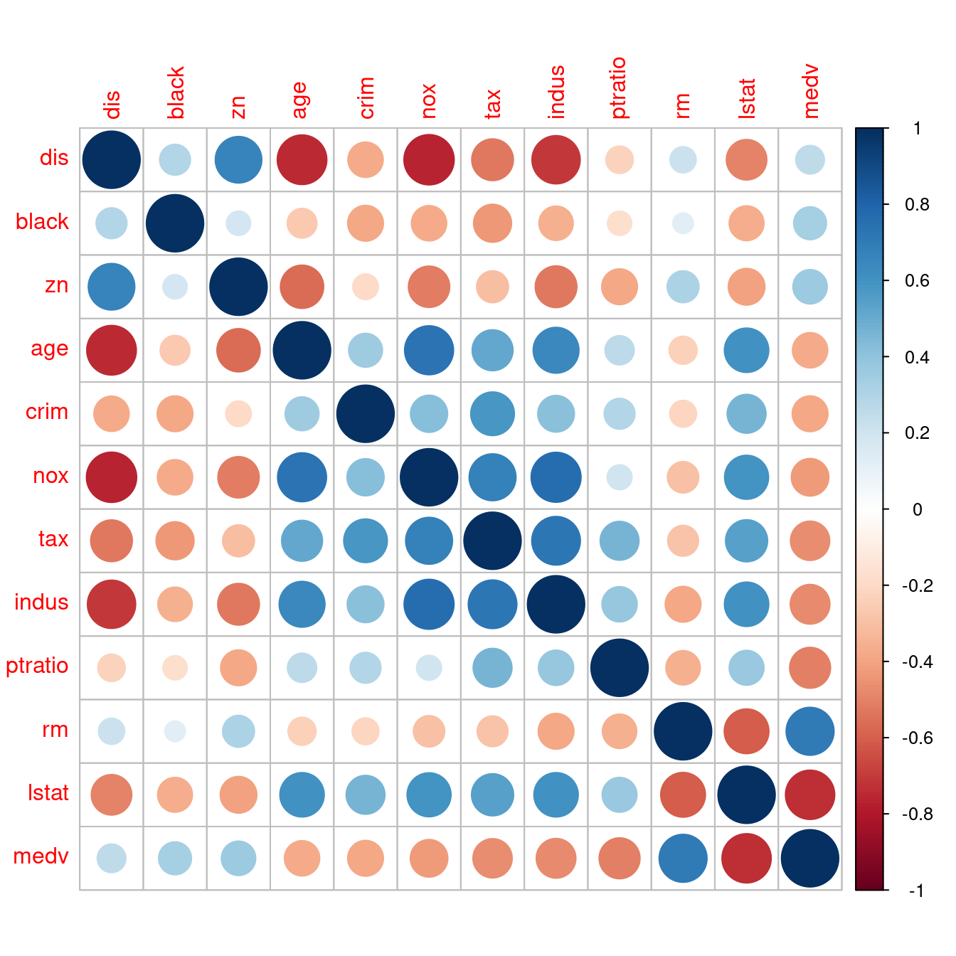
16.5.2 相關係數圖
「視覺化」相關係數矩陣是趨勢,原因是,實務上上述「相關係數矩陣」都很大,於是乎,統計學家再度出動,撰寫了套件「corrplot」。讓作者小編告訴大家如何用在波士頓數據集的相關係數矩陣:
- 呼叫套件「
corrplot」。
require(corrplot)- 準備波士頓數據集內連續型變數的相關係數矩陣。
corr <- round(cor(boston[, CONvars]), 2)- 問題:可以根據與房價中位數的相關係數大小排序嗎?因為「房價中位數」是第十二個變數,所以在「列方向」與「行方向」都加一句「
order(corr[12,])」,就可以維持「相關係數矩陣是對稱的」這一項性質。請讀者諸君專注在「最後一列」跟「最後一行」。完美!而且我們可以很輕鬆知道「全部連續型變數(lstat, ptratio, indus, tax, nox, crim, age, dis, black, zn, rm, medv)」與「房價中位數」的相關係數的「排行榜」!當然也可以有「按相關係數數值大小的排行榜」!作者小編認為第二個排行榜應該有助於「多個x變數的建模策略」,將在第八章實作、實驗這一項臆測!
corr <- corr[order(abs(corr[12,])), order(abs(corr[12,]))]
corrplot(corr)
16.5.3 回顧房價中位數與其他連續型變數的相關係數
繼續搜尋「房價中位數」的最小平方法迴歸線之前,先讓我們再一次回顧以下這幾個波士頓數據集內的連續型變數跟「房價中位數」的相關係數:
cor(x = boston[, CONvars[-12]], y = boston[, "medv"])## [,1]
## crim -0.3883046
## zn 0.3604453
## indus -0.4837252
## nox -0.4273208
## rm 0.6953599
## age -0.3769546
## dis 0.2499287
## tax -0.4685359
## ptratio -0.5077867
## black 0.3334608
## lstat -0.7376627我們發現
CORmedv <- cor(x = boston[, CONvars[-12]], y = boston[, "medv"])
rownames(CORmedv)[which(abs(CORmedv[,1]) <= 0.3)] # 小於0.3。
## [1] "dis"rownames(CORmedv)[which(abs(CORmedv[,1]) > 0.3 & abs(CORmedv[,1]) <= 0.5)] # 大於0.3且小於0.5。## [1] "crim" "zn" "indus" "nox" "age" "tax" "black"rownames(CORmedv)[which(abs(CORmedv[,1]) > 0.5 & abs(CORmedv[,1]) <= 0.7)] # 大於0.5且小於0.7。## [1] "rm" "ptratio"rownames(CORmedv)[which(abs(CORmedv[,1]) > 0.7)] # 大於0.7。## [1] "lstat"也發現
rownames(CORmedv)[which.max(abs(CORmedv[,1]))] # 最大相關係數發生在哪一個變數?## [1] "lstat"rownames(CORmedv)[which.min(abs(CORmedv[,1]))] # 最小相關係數發生在哪一個變數?## [1] "dis"因為這個發現,作者小編寫了這一段程式碼示範「中文版說明『colsBostonFull』的用途與用處」。
maxCOR <- rownames(CORmedv)[which.max(abs(CORmedv[,1]))]
plot(boston[, maxCOR], boston[, "medv"],
     xlab = colsBostonFull$中文變數名稱[which(colsBostonFull$變數名 == maxCOR)],
     ylab = "房價中位數")
title(paste0("最高相關係數", " = ",
             cor(boston[, maxCOR],
                 boston[, "medv"])))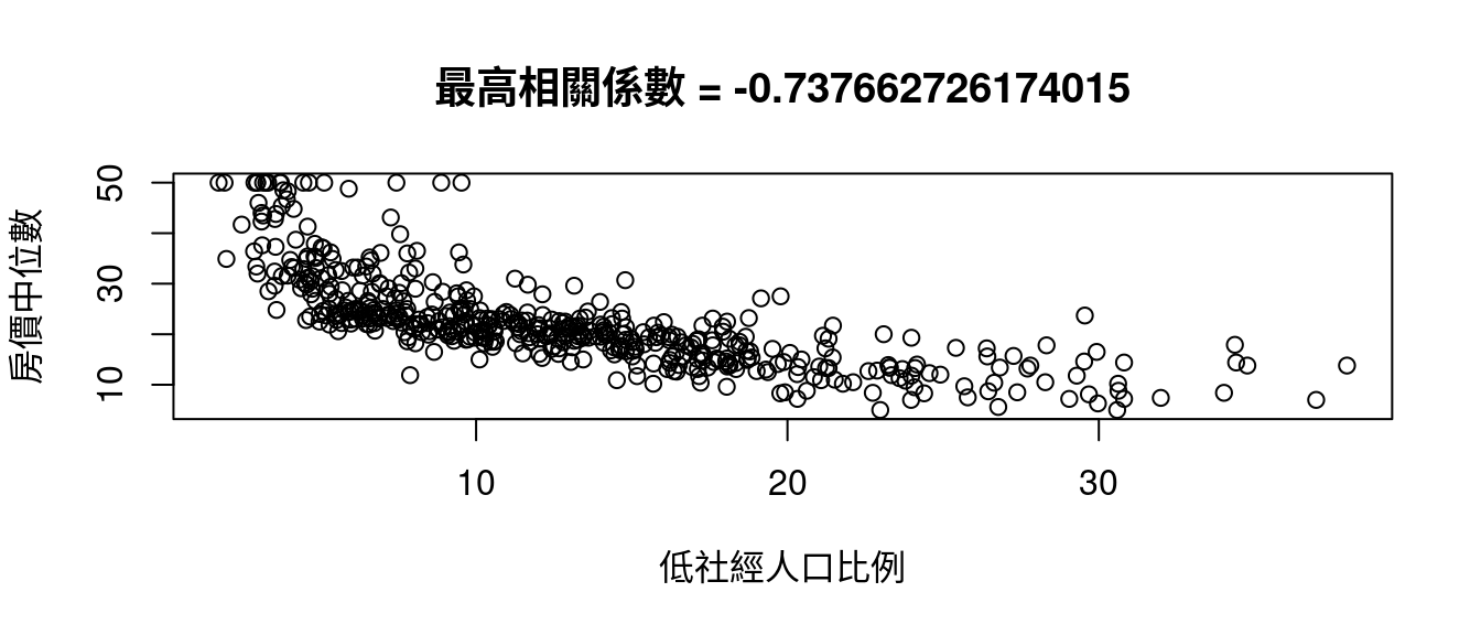
跟
minCOR <- rownames(CORmedv)[which.min(abs(CORmedv[,1]))]
plot(boston[, minCOR], boston[, "medv"],
     xlab = colsBostonFull$中文變數名稱[which(colsBostonFull$變數名 == minCOR)],
     ylab = "房價中位數")
title(paste0("最低相關係數", " = ",
             cor(boston[, minCOR],
                 boston[, "medv"])))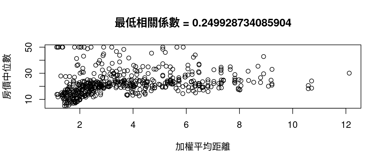
16.6 LS
16.6.2 第一個房價中位數的複迴歸模型
require(dplyr)
lm(medv ~ lstat, data = boston) %>%
  summary()
##
## Call:
## lm(formula = medv ~ lstat, data = boston)
##
## Residuals:
## Min 1Q Median 3Q Max
## -15.168 -3.990 -1.318 2.034 24.500
##
## Coefficients:
## Estimate Std. Error t value Pr(>|t|)
## (Intercept) 34.55384 0.56263 61.41 <0.0000000000000002 ***
## lstat -0.95005 0.03873 -24.53 <0.0000000000000002 ***
## ---
## Signif. codes: 0 '***' 0.001 '**' 0.01 '*' 0.05 '.' 0.1 ' ' 1
##
## Residual standard error: 6.216 on 504 degrees of freedom
## Multiple R-squared: 0.5441, Adjusted R-squared: 0.5432
## F-statistic: 601.6 on 1 and 504 DF, p-value: < 0.00000000000000022lm(medv ~ poly(lstat, 6, raw = TRUE), data = boston) %>%
summary()##
## Call:
## lm(formula = medv ~ poly(lstat, 6, raw = TRUE), data = boston)
##
## Residuals:
## Min 1Q Median 3Q Max
## -14.7317 -3.1571 -0.6941 2.0756 26.8994
##
## Coefficients:
## Estimate Std. Error t value
## (Intercept) 73.0433518598 5.5933680650 13.059
## poly(lstat, 6, raw = TRUE)1 -15.1673265415 2.9654385860 -5.115
## poly(lstat, 6, raw = TRUE)2 1.9295909151 0.5712522965 3.378
## poly(lstat, 6, raw = TRUE)3 -0.1307066978 0.0520184925 -2.513
## poly(lstat, 6, raw = TRUE)4 0.0046860540 0.0024065100 1.947
## poly(lstat, 6, raw = TRUE)5 -0.0000841615 0.0000545034 -1.544
## poly(lstat, 6, raw = TRUE)6 0.0000005974 0.0000004783 1.249
## Pr(>|t|)
## (Intercept) < 0.0000000000000002 ***
## poly(lstat, 6, raw = TRUE)1 0.000000449 ***
## poly(lstat, 6, raw = TRUE)2 0.000788 ***
## poly(lstat, 6, raw = TRUE)3 0.012295 *
## poly(lstat, 6, raw = TRUE)4 0.052066 .
## poly(lstat, 6, raw = TRUE)5 0.123186
## poly(lstat, 6, raw = TRUE)6 0.212313
## ---
## Signif. codes: 0 '***' 0.001 '**' 0.01 '*' 0.05 '.' 0.1 ' ' 1
##
## Residual standard error: 5.212 on 499 degrees of freedom
## Multiple R-squared: 0.6827, Adjusted R-squared: 0.6789
## F-statistic: 178.9 on 6 and 499 DF, p-value: < 0.00000000000000022lm(medv ~ lstat + ptratio, data = boston) %>%
summary()##
## Call:
## lm(formula = medv ~ lstat + ptratio, data = boston)
##
## Residuals:
## Min 1Q Median 3Q Max
## -12.2428 -3.6398 -0.8622 1.8790 26.9036
##
## Coefficients:
## Estimate Std. Error t value Pr(>|t|)
## (Intercept) 54.04682 2.24217 24.105 <0.0000000000000002 ***
## lstat -0.82018 0.03883 -21.120 <0.0000000000000002 ***
## ptratio -1.14525 0.12810 -8.941 <0.0000000000000002 ***
## ---
## Signif. codes: 0 '***' 0.001 '**' 0.01 '*' 0.05 '.' 0.1 ' ' 1
##
## Residual standard error: 5.78 on 503 degrees of freedom
## Multiple R-squared: 0.6067, Adjusted R-squared: 0.6051
## F-statistic: 387.9 on 2 and 503 DF, p-value: < 0.00000000000000022lm(medv ~ poly(lstat, 6, raw = TRUE) + ptratio, data = boston) %>%
summary()##
## Call:
## lm(formula = medv ~ poly(lstat, 6, raw = TRUE) + ptratio, data = boston)
##
## Residuals:
## Min 1Q Median 3Q Max
## -12.359 -2.722 -0.598 2.109 28.733
##
## Coefficients:
## Estimate Std. Error t value
## (Intercept) 83.8072130728 5.4748670192 15.308
## poly(lstat, 6, raw = TRUE)1 -13.1732525829 2.8182104559 -4.674
## poly(lstat, 6, raw = TRUE)2 1.5779214425 0.5425190942 2.909
## poly(lstat, 6, raw = TRUE)3 -0.0988372807 0.0494003548 -2.001
## poly(lstat, 6, raw = TRUE)4 0.0032401256 0.0022850813 1.418
## poly(lstat, 6, raw = TRUE)5 -0.0000528671 0.0000517381 -1.022
## poly(lstat, 6, raw = TRUE)6 0.0000003403 0.0000004539 0.750
## ptratio -0.8705960601 0.1131402463 -7.695
## Pr(>|t|)
## (Intercept) < 0.0000000000000002 ***
## poly(lstat, 6, raw = TRUE)1 0.0000038018112704 ***
## poly(lstat, 6, raw = TRUE)2 0.00379 **
## poly(lstat, 6, raw = TRUE)3 0.04596 *
## poly(lstat, 6, raw = TRUE)4 0.15683
## poly(lstat, 6, raw = TRUE)5 0.30736
## poly(lstat, 6, raw = TRUE)6 0.45380
## ptratio 0.0000000000000766 ***
## ---
## Signif. codes: 0 '***' 0.001 '**' 0.01 '*' 0.05 '.' 0.1 ' ' 1
##
## Residual standard error: 4.932 on 498 degrees of freedom
## Multiple R-squared: 0.7164, Adjusted R-squared: 0.7124
## F-statistic: 179.7 on 7 and 498 DF, p-value: < 0.00000000000000022lm(medv ~ poly(lstat, 6, raw = TRUE) + poly(ptratio, 6, raw = TRUE),
data = boston) %>%
summary()##
## Call:
## lm(formula = medv ~ poly(lstat, 6, raw = TRUE) + poly(ptratio,
## 6, raw = TRUE), data = boston)
##
## Residuals:
## Min 1Q Median 3Q Max
## -13.2375 -2.6692 -0.5043 2.1510 29.0361
##
## Coefficients:
## Estimate Std. Error t value
## (Intercept) -174559.5256428982 37070.9569862983 -4.709
## poly(lstat, 6, raw = TRUE)1 -12.8377019607 2.7345642099 -4.695
## poly(lstat, 6, raw = TRUE)2 1.4987970190 0.5244286840 2.858
## poly(lstat, 6, raw = TRUE)3 -0.0914306182 0.0476217933 -1.920
## poly(lstat, 6, raw = TRUE)4 0.0029116488 0.0021989208 1.324
## poly(lstat, 6, raw = TRUE)5 -0.0000458817 0.0000497277 -0.923
## poly(lstat, 6, raw = TRUE)6 0.0000002827 0.0000004359 0.649
## poly(ptratio, 6, raw = TRUE)1 61916.6871462194 13125.2665306501 4.717
## poly(ptratio, 6, raw = TRUE)2 -9075.6074431613 1924.2977504723 -4.716
## poly(ptratio, 6, raw = TRUE)3 704.1847388188 149.5632093646 4.708
## poly(ptratio, 6, raw = TRUE)4 -30.5149815826 6.5010099245 -4.694
## poly(ptratio, 6, raw = TRUE)5 0.7004432313 0.1498665972 4.674
## poly(ptratio, 6, raw = TRUE)6 -0.0066556993 0.0014317656 -4.649
## Pr(>|t|)
## (Intercept) 0.00000324 ***
## poly(lstat, 6, raw = TRUE)1 0.00000347 ***
## poly(lstat, 6, raw = TRUE)2 0.00444 **
## poly(lstat, 6, raw = TRUE)3 0.05544 .
## poly(lstat, 6, raw = TRUE)4 0.18607
## poly(lstat, 6, raw = TRUE)5 0.35664
## poly(lstat, 6, raw = TRUE)6 0.51688
## poly(ptratio, 6, raw = TRUE)1 0.00000312 ***
## poly(ptratio, 6, raw = TRUE)2 0.00000313 ***
## poly(ptratio, 6, raw = TRUE)3 0.00000325 ***
## poly(ptratio, 6, raw = TRUE)4 0.00000348 ***
## poly(ptratio, 6, raw = TRUE)5 0.00000382 ***
## poly(ptratio, 6, raw = TRUE)6 0.00000430 ***
## ---
## Signif. codes: 0 '***' 0.001 '**' 0.01 '*' 0.05 '.' 0.1 ' ' 1
##
## Residual standard error: 4.713 on 493 degrees of freedom
## Multiple R-squared: 0.7436, Adjusted R-squared: 0.7374
## F-statistic: 119.2 on 12 and 493 DF, p-value: < 0.00000000000000022lm(medv ~ poly(lstat, 6, raw = TRUE) + poly(ptratio, 8, raw = TRUE),
data = boston) %>%
summary()##
## Call:
## lm(formula = medv ~ poly(lstat, 6, raw = TRUE) + poly(ptratio,
## 8, raw = TRUE), data = boston)
##
## Residuals:
## Min 1Q Median 3Q Max
## -13.2063 -2.6652 -0.5787 2.1560 28.9593
##
## Coefficients: (1 not defined because of singularities)
## Estimate Std. Error t value
## (Intercept) -305922.6705500266 207506.1721243158 -1.474
## poly(lstat, 6, raw = TRUE)1 -12.9424987065 2.7410342501 -4.722
## poly(lstat, 6, raw = TRUE)2 1.5148686131 0.5253348136 2.884
## poly(lstat, 6, raw = TRUE)3 -0.0925284128 0.0476806583 -1.941
## poly(lstat, 6, raw = TRUE)4 0.0029473899 0.0022009300 1.339
## poly(lstat, 6, raw = TRUE)5 -0.0000464040 0.0000497640 -0.932
## poly(lstat, 6, raw = TRUE)6 0.0000002852 0.0000004362 0.654
## poly(ptratio, 8, raw = TRUE)1 116579.8406297475 85966.2970334381 1.356
## poly(ptratio, 8, raw = TRUE)2 -18768.1876719269 15186.7133233719 -1.236
## poly(ptratio, 8, raw = TRUE)3 1653.5708603829 1483.1008814656 1.115
## poly(ptratio, 8, raw = TRUE)4 -85.9985686322 86.4773157437 -0.994
## poly(ptratio, 8, raw = TRUE)5 2.6352844512 3.0108573046 0.875
## poly(ptratio, 8, raw = TRUE)6 -0.0439383878 0.0579622785 -0.758
## poly(ptratio, 8, raw = TRUE)7 0.0003062638 0.0004759936 0.643
## poly(ptratio, 8, raw = TRUE)8 NA NA NA
## Pr(>|t|)
## (Intercept) 0.1410
## poly(lstat, 6, raw = TRUE)1 0.00000305 ***
## poly(lstat, 6, raw = TRUE)2 0.0041 **
## poly(lstat, 6, raw = TRUE)3 0.0529 .
## poly(lstat, 6, raw = TRUE)4 0.1811
## poly(lstat, 6, raw = TRUE)5 0.3515
## poly(lstat, 6, raw = TRUE)6 0.5134
## poly(ptratio, 8, raw = TRUE)1 0.1757
## poly(ptratio, 8, raw = TRUE)2 0.2171
## poly(ptratio, 8, raw = TRUE)3 0.2654
## poly(ptratio, 8, raw = TRUE)4 0.3205
## poly(ptratio, 8, raw = TRUE)5 0.3819
## poly(ptratio, 8, raw = TRUE)6 0.4488
## poly(ptratio, 8, raw = TRUE)7 0.5203
## poly(ptratio, 8, raw = TRUE)8 NA
## ---
## Signif. codes: 0 '***' 0.001 '**' 0.01 '*' 0.05 '.' 0.1 ' ' 1
##
## Residual standard error: 4.716 on 492 degrees of freedom
## Multiple R-squared: 0.7438, Adjusted R-squared: 0.7371
## F-statistic: 109.9 on 13 and 492 DF, p-value: < 0.0000000000000002216.6.3 第一個房價中位數複迴歸模型的最佳解
lm(medv ~ poly(lstat, 6, raw = TRUE) + poly(ptratio, 6, raw = TRUE),
          data = boston) %>%
  summary()
##
## Call:
## lm(formula = medv ~ poly(lstat, 6, raw = TRUE) + poly(ptratio,
## 6, raw = TRUE), data = boston)
##
## Residuals:
## Min 1Q Median 3Q Max
## -13.2375 -2.6692 -0.5043 2.1510 29.0361
##
## Coefficients:
## Estimate Std. Error t value
## (Intercept) -174559.5256428982 37070.9569862983 -4.709
## poly(lstat, 6, raw = TRUE)1 -12.8377019607 2.7345642099 -4.695
## poly(lstat, 6, raw = TRUE)2 1.4987970190 0.5244286840 2.858
## poly(lstat, 6, raw = TRUE)3 -0.0914306182 0.0476217933 -1.920
## poly(lstat, 6, raw = TRUE)4 0.0029116488 0.0021989208 1.324
## poly(lstat, 6, raw = TRUE)5 -0.0000458817 0.0000497277 -0.923
## poly(lstat, 6, raw = TRUE)6 0.0000002827 0.0000004359 0.649
## poly(ptratio, 6, raw = TRUE)1 61916.6871462194 13125.2665306501 4.717
## poly(ptratio, 6, raw = TRUE)2 -9075.6074431613 1924.2977504723 -4.716
## poly(ptratio, 6, raw = TRUE)3 704.1847388188 149.5632093646 4.708
## poly(ptratio, 6, raw = TRUE)4 -30.5149815826 6.5010099245 -4.694
## poly(ptratio, 6, raw = TRUE)5 0.7004432313 0.1498665972 4.674
## poly(ptratio, 6, raw = TRUE)6 -0.0066556993 0.0014317656 -4.649
## Pr(>|t|)
## (Intercept) 0.00000324 ***
## poly(lstat, 6, raw = TRUE)1 0.00000347 ***
## poly(lstat, 6, raw = TRUE)2 0.00444 **
## poly(lstat, 6, raw = TRUE)3 0.05544 .
## poly(lstat, 6, raw = TRUE)4 0.18607
## poly(lstat, 6, raw = TRUE)5 0.35664
## poly(lstat, 6, raw = TRUE)6 0.51688
## poly(ptratio, 6, raw = TRUE)1 0.00000312 ***
## poly(ptratio, 6, raw = TRUE)2 0.00000313 ***
## poly(ptratio, 6, raw = TRUE)3 0.00000325 ***
## poly(ptratio, 6, raw = TRUE)4 0.00000348 ***
## poly(ptratio, 6, raw = TRUE)5 0.00000382 ***
## poly(ptratio, 6, raw = TRUE)6 0.00000430 ***
## ---
## Signif. codes: 0 '***' 0.001 '**' 0.01 '*' 0.05 '.' 0.1 ' ' 1
##
## Residual standard error: 4.713 on 493 degrees of freedom
## Multiple R-squared: 0.7436, Adjusted R-squared: 0.7374
## F-statistic: 119.2 on 12 and 493 DF, p-value: < 0.0000000000000002216.7 再看一次波士頓數據集的全貌散佈圖談提升\(R^2\)
require(caret)
featurePlot(x = boston[, CONvars[-12]],
            y = boston$medv,
            plot = "scatter",
            type = c("p", "smooth"), col = "blue")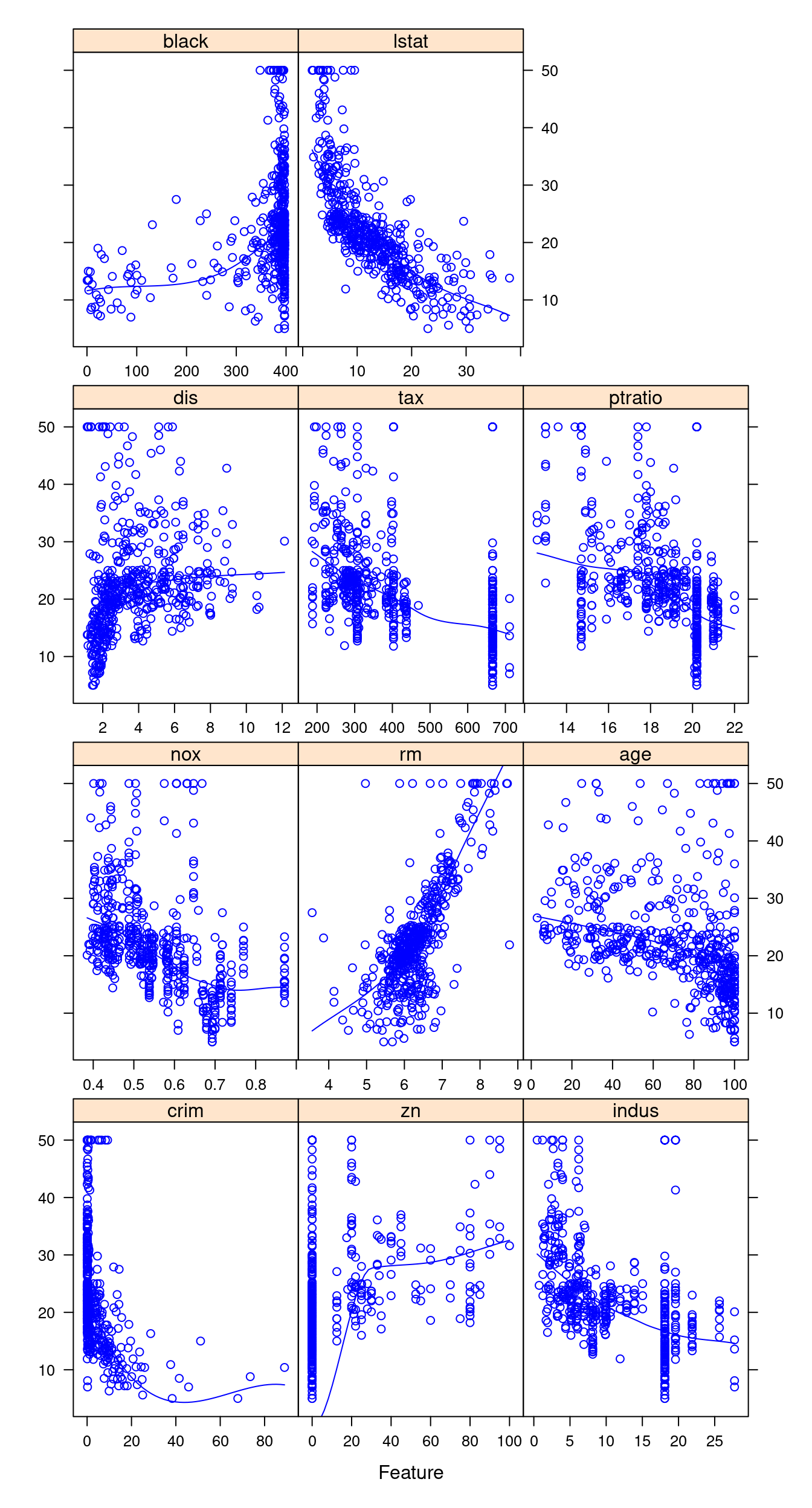
16.7.1 多項式迴歸模型
dropList <- c('chas','rad','crim','zn','black')
# We drop chas and rad because they are non numeric
# We drop crim, zn and black because they have lot of outliers
housing <- boston[,!colnames(boston) %in% dropList]

# Fitting Simple Linear regression
# . is used to fit predictor using all independent variables
lm.fit1 <- lm(medv ~ ., data = housing)
summary(lm.fit1)
##
## Call:
## lm(formula = medv ~ ., data = housing)
##
## Residuals:
## Min 1Q Median 3Q Max
## -12.6429 -2.9278 -0.7301 1.9617 28.0761
##
## Coefficients:
## Estimate Std. Error t value Pr(>|t|)
## (Intercept) 36.5879716 4.8574379 7.532 0.0000000000002370 ***
## indus -0.0391358 0.0613975 -0.637 0.524
## nox -16.0859041 3.9623819 -4.060 0.0000570790474413 ***
## rm 4.1593303 0.4270941 9.739 < 0.0000000000000002 ***
## age -0.0019644 0.0137462 -0.143 0.886
## dis -1.2246809 0.1909527 -6.414 0.0000000003314073 ***
## tax -0.0008703 0.0021660 -0.402 0.688
## ptratio -1.0002112 0.1270260 -7.874 0.0000000000000217 ***
## lstat -0.5721361 0.0515402 -11.101 < 0.0000000000000002 ***
## ---
## Signif. codes: 0 '***' 0.001 '**' 0.01 '*' 0.05 '.' 0.1 ' ' 1
##
## Residual standard error: 5.005 on 497 degrees of freedom
## Multiple R-squared: 0.7086, Adjusted R-squared: 0.7039
## F-statistic: 151.1 on 8 and 497 DF, p-value: < 0.00000000000000022lm.fit2 <- lm(medv ~ . -age -indus -tax, data = housing)
summary(lm.fit2)##
## Call:
## lm(formula = medv ~ . - age - indus - tax, data = housing)
##
## Residuals:
## Min 1Q Median 3Q Max
## -12.7765 -3.0186 -0.6481 1.9752 27.7625
##
## Coefficients:
## Estimate Std. Error t value Pr(>|t|)
## (Intercept) 37.49920 4.61295 8.129 0.00000000000000343 ***
## nox -17.99657 3.26095 -5.519 0.00000005488148102 ***
## rm 4.16331 0.41203 10.104 < 0.0000000000000002 ***
## dis -1.18466 0.16842 -7.034 0.00000000000664218 ***
## ptratio -1.04577 0.11352 -9.212 < 0.0000000000000002 ***
## lstat -0.58108 0.04794 -12.122 < 0.0000000000000002 ***
## ---
## Signif. codes: 0 '***' 0.001 '**' 0.01 '*' 0.05 '.' 0.1 ' ' 1
##
## Residual standard error: 4.994 on 500 degrees of freedom
## Multiple R-squared: 0.7081, Adjusted R-squared: 0.7052
## F-statistic: 242.6 on 5 and 500 DF, p-value: < 0.00000000000000022lm.fit3 <- lm(medv ~ . -age -indus -tax +I(lstat^2), data = housing)
summary(lm.fit3)##
## Call:
## lm(formula = medv ~ . - age - indus - tax + I(lstat^2), data = housing)
##
## Residuals:
## Min 1Q Median 3Q Max
## -14.5160 -2.9156 -0.2918 2.1449 26.4922
##
## Coefficients:
## Estimate Std. Error t value Pr(>|t|)
## (Intercept) 43.654445 4.257579 10.253 < 0.0000000000000002 ***
## nox -13.833488 3.007086 -4.600 0.0000053559578082 ***
## rm 3.433253 0.383295 8.957 < 0.0000000000000002 ***
## dis -1.202378 0.153833 -7.816 0.0000000000000325 ***
## ptratio -0.836542 0.105759 -7.910 0.0000000000000167 ***
## lstat -1.735731 0.123257 -14.082 < 0.0000000000000002 ***
## I(lstat^2) 0.032888 0.003282 10.021 < 0.0000000000000002 ***
## ---
## Signif. codes: 0 '***' 0.001 '**' 0.01 '*' 0.05 '.' 0.1 ' ' 1
##
## Residual standard error: 4.561 on 499 degrees of freedom
## Multiple R-squared: 0.757, Adjusted R-squared: 0.7541
## F-statistic: 259.1 on 6 and 499 DF, p-value: < 0.00000000000000022