Chapter 17 當複線性迴歸遇上機器學習
17.3 準備工作
17.3.1 波士頓數據集
require(MASS) # 用「require」不用「library」,是因為如果R已經將套件MASS載入環境,就不需要再載一次。
data(Boston)
boston <- Boston
# 「不動」原始數據集,不論它有「多原始」,是R程式設計的一項絕佳習慣。
# 即便一般使用者是無法任意改變套件MASS的內容物!
### rad (index of accessibility to radial highways)
boston[,"rad"] <- factor(boston[,"rad"], ordered = TRUE)
### chas (= 1 if tract bounds river; 0 otherwise)
boston[,"chas"] <- factor(boston[,"chas"])
head(boston)
## crim zn indus chas nox rm age dis rad tax ptratio black lstat
## 1 0.00632 18 2.31 0 0.538 6.575 65.2 4.0900 1 296 15.3 396.90 4.98
## 2 0.02731 0 7.07 0 0.469 6.421 78.9 4.9671 2 242 17.8 396.90 9.14
## 3 0.02729 0 7.07 0 0.469 7.185 61.1 4.9671 2 242 17.8 392.83 4.03
## 4 0.03237 0 2.18 0 0.458 6.998 45.8 6.0622 3 222 18.7 394.63 2.94
## 5 0.06905 0 2.18 0 0.458 7.147 54.2 6.0622 3 222 18.7 396.90 5.33
## 6 0.02985 0 2.18 0 0.458 6.430 58.7 6.0622 3 222 18.7 394.12 5.21
## medv
## 1 24.0
## 2 21.6
## 3 34.7
## 4 33.4
## 5 36.2
## 6 28.7tail(boston)## crim zn indus chas nox rm age dis rad tax ptratio black lstat
## 501 0.22438 0 9.69 0 0.585 6.027 79.7 2.4982 6 391 19.2 396.90 14.33
## 502 0.06263 0 11.93 0 0.573 6.593 69.1 2.4786 1 273 21.0 391.99 9.67
## 503 0.04527 0 11.93 0 0.573 6.120 76.7 2.2875 1 273 21.0 396.90 9.08
## 504 0.06076 0 11.93 0 0.573 6.976 91.0 2.1675 1 273 21.0 396.90 5.64
## 505 0.10959 0 11.93 0 0.573 6.794 89.3 2.3889 1 273 21.0 393.45 6.48
## 506 0.04741 0 11.93 0 0.573 6.030 80.8 2.5050 1 273 21.0 396.90 7.88
## medv
## 501 16.8
## 502 22.4
## 503 20.6
## 504 23.9
## 505 22.0
## 506 11.9### 讀取自製的波士頓數據集中文資訊。
DISvars <- colnames(boston)[which(sapply(boston, class) == "integer")]
CONvars <- colnames(boston)[which(sapply(boston, class) == "numeric")]
colsBostonFull<-readRDS("output/data/colsBostonFull.rds")
colsBostonFull$內容物 <- sapply(boston, class)
colsBostonFull## 變數名
## 1 crim
## 2 zn
## 3 indus
## 4 chas
## 5 nox
## 6 rm
## 7 age
## 8 dis
## 9 rad
## 10 tax
## 11 ptratio
## 12 black
## 13 lstat
## 14 medv
## 說明
## 1 per capita crime rate by town
## 2 proportion of residential land zoned for lots over 25,000 sq.ft.
## 3 proportion of non-retail business acres per town
## 4 Charles River dummy variable (= 1 if tract bounds river; 0 otherwise)
## 5 nitric oxides concentration (parts per 10 million)
## 6 average number of rooms per dwelling
## 7 proportion of owner-occupied units built prior to 1940
## 8 weighted distances to five Boston employment centres
## 9 index of accessibility to radial highways
## 10 full-value property-tax rate per $10,000
## 11 pupil-teacher ratio by town
## 12 1000(Bk - 0.63)^2 where Bk is the proportion of blacks by town
## 13 % lower status of the population
## 14 Median value of owner-occupied homes in $1000's
## 中文翻譯 中文變數名稱 內容物
## 1 每個城鎮人均犯罪率。 犯罪率 numeric
## 2 超過25,000平方呎的住宅用地比例。 住宅用地比例 numeric
## 3 每個城鎮非零售業務英畝的比例。 非商業區比例 numeric
## 4 是否鄰近Charles River。 河邊宅 factor
## 5 氮氧化合物濃度。 空汙指標 numeric
## 6 每個住宅的平均房間數。 平均房間數 numeric
## 7 1940年之前建造的自用住宅比例。 老房子比例 numeric
## 8 距波士頓五大商圈的加權平均距離。 加權平均距離 numeric
## 9 環狀高速公路的可觸指標。 交通便利性 ordered, factor
## 10 財產稅占比(每一萬美元)。 財產稅率 numeric
## 11 生師比。 生師比 numeric
## 12 黑人的比例。 黑人指數 numeric
## 13 (比較)低社經地位人口的比例。 低社經人口比例 numeric
## 14 以千美元計的房價中位數。 房價中位數 numeric17.4 LS
17.4.2 第一個房價中位數的複迴歸模型
require(dplyr)
lm(medv ~ lstat, data = boston) %>%
  summary()
##
## Call:
## lm(formula = medv ~ lstat, data = boston)
##
## Residuals:
## Min 1Q Median 3Q Max
## -15.168 -3.990 -1.318 2.034 24.500
##
## Coefficients:
## Estimate Std. Error t value Pr(>|t|)
## (Intercept) 34.55384 0.56263 61.41 <0.0000000000000002 ***
## lstat -0.95005 0.03873 -24.53 <0.0000000000000002 ***
## ---
## Signif. codes: 0 '***' 0.001 '**' 0.01 '*' 0.05 '.' 0.1 ' ' 1
##
## Residual standard error: 6.216 on 504 degrees of freedom
## Multiple R-squared: 0.5441, Adjusted R-squared: 0.5432
## F-statistic: 601.6 on 1 and 504 DF, p-value: < 0.00000000000000022lm(medv ~ poly(lstat, 6, raw = TRUE), data = boston) %>%
summary()##
## Call:
## lm(formula = medv ~ poly(lstat, 6, raw = TRUE), data = boston)
##
## Residuals:
## Min 1Q Median 3Q Max
## -14.7317 -3.1571 -0.6941 2.0756 26.8994
##
## Coefficients:
## Estimate Std. Error t value
## (Intercept) 73.0433518598 5.5933680650 13.059
## poly(lstat, 6, raw = TRUE)1 -15.1673265415 2.9654385860 -5.115
## poly(lstat, 6, raw = TRUE)2 1.9295909151 0.5712522965 3.378
## poly(lstat, 6, raw = TRUE)3 -0.1307066978 0.0520184925 -2.513
## poly(lstat, 6, raw = TRUE)4 0.0046860540 0.0024065100 1.947
## poly(lstat, 6, raw = TRUE)5 -0.0000841615 0.0000545034 -1.544
## poly(lstat, 6, raw = TRUE)6 0.0000005974 0.0000004783 1.249
## Pr(>|t|)
## (Intercept) < 0.0000000000000002 ***
## poly(lstat, 6, raw = TRUE)1 0.000000449 ***
## poly(lstat, 6, raw = TRUE)2 0.000788 ***
## poly(lstat, 6, raw = TRUE)3 0.012295 *
## poly(lstat, 6, raw = TRUE)4 0.052066 .
## poly(lstat, 6, raw = TRUE)5 0.123186
## poly(lstat, 6, raw = TRUE)6 0.212313
## ---
## Signif. codes: 0 '***' 0.001 '**' 0.01 '*' 0.05 '.' 0.1 ' ' 1
##
## Residual standard error: 5.212 on 499 degrees of freedom
## Multiple R-squared: 0.6827, Adjusted R-squared: 0.6789
## F-statistic: 178.9 on 6 and 499 DF, p-value: < 0.00000000000000022lm(medv ~ lstat + ptratio, data = boston) %>%
summary()##
## Call:
## lm(formula = medv ~ lstat + ptratio, data = boston)
##
## Residuals:
## Min 1Q Median 3Q Max
## -12.2428 -3.6398 -0.8622 1.8790 26.9036
##
## Coefficients:
## Estimate Std. Error t value Pr(>|t|)
## (Intercept) 54.04682 2.24217 24.105 <0.0000000000000002 ***
## lstat -0.82018 0.03883 -21.120 <0.0000000000000002 ***
## ptratio -1.14525 0.12810 -8.941 <0.0000000000000002 ***
## ---
## Signif. codes: 0 '***' 0.001 '**' 0.01 '*' 0.05 '.' 0.1 ' ' 1
##
## Residual standard error: 5.78 on 503 degrees of freedom
## Multiple R-squared: 0.6067, Adjusted R-squared: 0.6051
## F-statistic: 387.9 on 2 and 503 DF, p-value: < 0.00000000000000022lm(medv ~ poly(lstat, 6, raw = TRUE) + ptratio, data = boston) %>%
summary()##
## Call:
## lm(formula = medv ~ poly(lstat, 6, raw = TRUE) + ptratio, data = boston)
##
## Residuals:
## Min 1Q Median 3Q Max
## -12.359 -2.722 -0.598 2.109 28.733
##
## Coefficients:
## Estimate Std. Error t value
## (Intercept) 83.8072130728 5.4748670192 15.308
## poly(lstat, 6, raw = TRUE)1 -13.1732525829 2.8182104559 -4.674
## poly(lstat, 6, raw = TRUE)2 1.5779214425 0.5425190942 2.909
## poly(lstat, 6, raw = TRUE)3 -0.0988372807 0.0494003548 -2.001
## poly(lstat, 6, raw = TRUE)4 0.0032401256 0.0022850813 1.418
## poly(lstat, 6, raw = TRUE)5 -0.0000528671 0.0000517381 -1.022
## poly(lstat, 6, raw = TRUE)6 0.0000003403 0.0000004539 0.750
## ptratio -0.8705960601 0.1131402463 -7.695
## Pr(>|t|)
## (Intercept) < 0.0000000000000002 ***
## poly(lstat, 6, raw = TRUE)1 0.0000038018112704 ***
## poly(lstat, 6, raw = TRUE)2 0.00379 **
## poly(lstat, 6, raw = TRUE)3 0.04596 *
## poly(lstat, 6, raw = TRUE)4 0.15683
## poly(lstat, 6, raw = TRUE)5 0.30736
## poly(lstat, 6, raw = TRUE)6 0.45380
## ptratio 0.0000000000000766 ***
## ---
## Signif. codes: 0 '***' 0.001 '**' 0.01 '*' 0.05 '.' 0.1 ' ' 1
##
## Residual standard error: 4.932 on 498 degrees of freedom
## Multiple R-squared: 0.7164, Adjusted R-squared: 0.7124
## F-statistic: 179.7 on 7 and 498 DF, p-value: < 0.00000000000000022lm(medv ~ poly(lstat, 6, raw = TRUE) +
poly(ptratio, 6, raw = TRUE),
data = boston) %>%
summary()##
## Call:
## lm(formula = medv ~ poly(lstat, 6, raw = TRUE) + poly(ptratio,
## 6, raw = TRUE), data = boston)
##
## Residuals:
## Min 1Q Median 3Q Max
## -13.2375 -2.6692 -0.5043 2.1510 29.0361
##
## Coefficients:
## Estimate Std. Error t value
## (Intercept) -174559.5256428982 37070.9569862983 -4.709
## poly(lstat, 6, raw = TRUE)1 -12.8377019607 2.7345642099 -4.695
## poly(lstat, 6, raw = TRUE)2 1.4987970190 0.5244286840 2.858
## poly(lstat, 6, raw = TRUE)3 -0.0914306182 0.0476217933 -1.920
## poly(lstat, 6, raw = TRUE)4 0.0029116488 0.0021989208 1.324
## poly(lstat, 6, raw = TRUE)5 -0.0000458817 0.0000497277 -0.923
## poly(lstat, 6, raw = TRUE)6 0.0000002827 0.0000004359 0.649
## poly(ptratio, 6, raw = TRUE)1 61916.6871462194 13125.2665306501 4.717
## poly(ptratio, 6, raw = TRUE)2 -9075.6074431613 1924.2977504723 -4.716
## poly(ptratio, 6, raw = TRUE)3 704.1847388188 149.5632093646 4.708
## poly(ptratio, 6, raw = TRUE)4 -30.5149815826 6.5010099245 -4.694
## poly(ptratio, 6, raw = TRUE)5 0.7004432313 0.1498665972 4.674
## poly(ptratio, 6, raw = TRUE)6 -0.0066556993 0.0014317656 -4.649
## Pr(>|t|)
## (Intercept) 0.00000324 ***
## poly(lstat, 6, raw = TRUE)1 0.00000347 ***
## poly(lstat, 6, raw = TRUE)2 0.00444 **
## poly(lstat, 6, raw = TRUE)3 0.05544 .
## poly(lstat, 6, raw = TRUE)4 0.18607
## poly(lstat, 6, raw = TRUE)5 0.35664
## poly(lstat, 6, raw = TRUE)6 0.51688
## poly(ptratio, 6, raw = TRUE)1 0.00000312 ***
## poly(ptratio, 6, raw = TRUE)2 0.00000313 ***
## poly(ptratio, 6, raw = TRUE)3 0.00000325 ***
## poly(ptratio, 6, raw = TRUE)4 0.00000348 ***
## poly(ptratio, 6, raw = TRUE)5 0.00000382 ***
## poly(ptratio, 6, raw = TRUE)6 0.00000430 ***
## ---
## Signif. codes: 0 '***' 0.001 '**' 0.01 '*' 0.05 '.' 0.1 ' ' 1
##
## Residual standard error: 4.713 on 493 degrees of freedom
## Multiple R-squared: 0.7436, Adjusted R-squared: 0.7374
## F-statistic: 119.2 on 12 and 493 DF, p-value: < 0.00000000000000022lm(medv ~ poly(lstat, 6, raw = TRUE) +
poly(ptratio, 8, raw = TRUE),
data = boston) %>%
summary()##
## Call:
## lm(formula = medv ~ poly(lstat, 6, raw = TRUE) + poly(ptratio,
## 8, raw = TRUE), data = boston)
##
## Residuals:
## Min 1Q Median 3Q Max
## -13.2063 -2.6652 -0.5787 2.1560 28.9593
##
## Coefficients: (1 not defined because of singularities)
## Estimate Std. Error t value
## (Intercept) -305922.6705500266 207506.1721243158 -1.474
## poly(lstat, 6, raw = TRUE)1 -12.9424987065 2.7410342501 -4.722
## poly(lstat, 6, raw = TRUE)2 1.5148686131 0.5253348136 2.884
## poly(lstat, 6, raw = TRUE)3 -0.0925284128 0.0476806583 -1.941
## poly(lstat, 6, raw = TRUE)4 0.0029473899 0.0022009300 1.339
## poly(lstat, 6, raw = TRUE)5 -0.0000464040 0.0000497640 -0.932
## poly(lstat, 6, raw = TRUE)6 0.0000002852 0.0000004362 0.654
## poly(ptratio, 8, raw = TRUE)1 116579.8406297475 85966.2970334381 1.356
## poly(ptratio, 8, raw = TRUE)2 -18768.1876719269 15186.7133233719 -1.236
## poly(ptratio, 8, raw = TRUE)3 1653.5708603829 1483.1008814656 1.115
## poly(ptratio, 8, raw = TRUE)4 -85.9985686322 86.4773157437 -0.994
## poly(ptratio, 8, raw = TRUE)5 2.6352844512 3.0108573046 0.875
## poly(ptratio, 8, raw = TRUE)6 -0.0439383878 0.0579622785 -0.758
## poly(ptratio, 8, raw = TRUE)7 0.0003062638 0.0004759936 0.643
## poly(ptratio, 8, raw = TRUE)8 NA NA NA
## Pr(>|t|)
## (Intercept) 0.1410
## poly(lstat, 6, raw = TRUE)1 0.00000305 ***
## poly(lstat, 6, raw = TRUE)2 0.0041 **
## poly(lstat, 6, raw = TRUE)3 0.0529 .
## poly(lstat, 6, raw = TRUE)4 0.1811
## poly(lstat, 6, raw = TRUE)5 0.3515
## poly(lstat, 6, raw = TRUE)6 0.5134
## poly(ptratio, 8, raw = TRUE)1 0.1757
## poly(ptratio, 8, raw = TRUE)2 0.2171
## poly(ptratio, 8, raw = TRUE)3 0.2654
## poly(ptratio, 8, raw = TRUE)4 0.3205
## poly(ptratio, 8, raw = TRUE)5 0.3819
## poly(ptratio, 8, raw = TRUE)6 0.4488
## poly(ptratio, 8, raw = TRUE)7 0.5203
## poly(ptratio, 8, raw = TRUE)8 NA
## ---
## Signif. codes: 0 '***' 0.001 '**' 0.01 '*' 0.05 '.' 0.1 ' ' 1
##
## Residual standard error: 4.716 on 492 degrees of freedom
## Multiple R-squared: 0.7438, Adjusted R-squared: 0.7371
## F-statistic: 109.9 on 13 and 492 DF, p-value: < 0.0000000000000002217.4.3 第一個房價中位數複迴歸模型的最佳解
lm(medv ~ poly(lstat, 6, raw = TRUE) +
     poly(ptratio, 6, raw = TRUE),
   data = boston) %>%
  summary()
##
## Call:
## lm(formula = medv ~ poly(lstat, 6, raw = TRUE) + poly(ptratio,
## 6, raw = TRUE), data = boston)
##
## Residuals:
## Min 1Q Median 3Q Max
## -13.2375 -2.6692 -0.5043 2.1510 29.0361
##
## Coefficients:
## Estimate Std. Error t value
## (Intercept) -174559.5256428982 37070.9569862983 -4.709
## poly(lstat, 6, raw = TRUE)1 -12.8377019607 2.7345642099 -4.695
## poly(lstat, 6, raw = TRUE)2 1.4987970190 0.5244286840 2.858
## poly(lstat, 6, raw = TRUE)3 -0.0914306182 0.0476217933 -1.920
## poly(lstat, 6, raw = TRUE)4 0.0029116488 0.0021989208 1.324
## poly(lstat, 6, raw = TRUE)5 -0.0000458817 0.0000497277 -0.923
## poly(lstat, 6, raw = TRUE)6 0.0000002827 0.0000004359 0.649
## poly(ptratio, 6, raw = TRUE)1 61916.6871462194 13125.2665306501 4.717
## poly(ptratio, 6, raw = TRUE)2 -9075.6074431613 1924.2977504723 -4.716
## poly(ptratio, 6, raw = TRUE)3 704.1847388188 149.5632093646 4.708
## poly(ptratio, 6, raw = TRUE)4 -30.5149815826 6.5010099245 -4.694
## poly(ptratio, 6, raw = TRUE)5 0.7004432313 0.1498665972 4.674
## poly(ptratio, 6, raw = TRUE)6 -0.0066556993 0.0014317656 -4.649
## Pr(>|t|)
## (Intercept) 0.00000324 ***
## poly(lstat, 6, raw = TRUE)1 0.00000347 ***
## poly(lstat, 6, raw = TRUE)2 0.00444 **
## poly(lstat, 6, raw = TRUE)3 0.05544 .
## poly(lstat, 6, raw = TRUE)4 0.18607
## poly(lstat, 6, raw = TRUE)5 0.35664
## poly(lstat, 6, raw = TRUE)6 0.51688
## poly(ptratio, 6, raw = TRUE)1 0.00000312 ***
## poly(ptratio, 6, raw = TRUE)2 0.00000313 ***
## poly(ptratio, 6, raw = TRUE)3 0.00000325 ***
## poly(ptratio, 6, raw = TRUE)4 0.00000348 ***
## poly(ptratio, 6, raw = TRUE)5 0.00000382 ***
## poly(ptratio, 6, raw = TRUE)6 0.00000430 ***
## ---
## Signif. codes: 0 '***' 0.001 '**' 0.01 '*' 0.05 '.' 0.1 ' ' 1
##
## Residual standard error: 4.713 on 493 degrees of freedom
## Multiple R-squared: 0.7436, Adjusted R-squared: 0.7374
## F-statistic: 119.2 on 12 and 493 DF, p-value: < 0.0000000000000002217.5 LASSO
df <- boston
y <- df[, "medv"]
X <- matrix(c(df[, "lstat"], df[, "ptratio"]),
            dim(df)[1],
            2,
            byrow = FALSE)
head(X)
## [,1] [,2]
## [1,] 4.98 15.3
## [2,] 9.14 17.8
## [3,] 4.03 17.8
## [4,] 2.94 18.7
## [5,] 5.33 18.7
## [6,] 5.21 18.7tail(X)## [,1] [,2]
## [501,] 14.33 19.2
## [502,] 9.67 21.0
## [503,] 9.08 21.0
## [504,] 5.64 21.0
## [505,] 6.48 21.0
## [506,] 7.88 21.0require(glmnet)
fit1 <- glmnet(X, y)
fit1##
## Call: glmnet(x = X, y = y)
##
## Df %Dev Lambda
## 1 0 0.00 6.7780
## 2 1 9.24 6.1760
## 3 1 16.91 5.6270
## 4 1 23.28 5.1270
## 5 1 28.56 4.6720
## 6 1 32.95 4.2570
## 7 1 36.60 3.8780
## 8 1 39.62 3.5340
## 9 2 42.79 3.2200
## 10 2 45.82 2.9340
## 11 2 48.34 2.6730
## 12 2 50.44 2.4360
## 13 2 52.17 2.2190
## 14 2 53.61 2.0220
## 15 2 54.81 1.8430
## 16 2 55.81 1.6790
## 17 2 56.63 1.5300
## 18 2 57.32 1.3940
## 19 2 57.88 1.2700
## 20 2 58.36 1.1570
## 21 2 58.75 1.0540
## 22 2 59.07 0.9607
## 23 2 59.34 0.8754
## 24 2 59.57 0.7976
## 25 2 59.75 0.7267
## 26 2 59.91 0.6622
## 27 2 60.04 0.6034
## 28 2 60.14 0.5498
## 29 2 60.23 0.5009
## 30 2 60.31 0.4564
## 31 2 60.37 0.4159
## 32 2 60.42 0.3789
## 33 2 60.46 0.3453
## 34 2 60.49 0.3146
## 35 2 60.52 0.2866
## 36 2 60.55 0.2612
## 37 2 60.57 0.2380
## 38 2 60.58 0.2168
## 39 2 60.60 0.1976
## 40 2 60.61 0.1800
## 41 2 60.62 0.1640
## 42 2 60.63 0.1495
## 43 2 60.63 0.1362
## 44 2 60.64 0.1241
## 45 2 60.64 0.1131
## 46 2 60.65 0.1030
## 47 2 60.65 0.0939
## 48 2 60.65 0.0855
## 49 2 60.65 0.0779
## 50 2 60.66 0.0710
## 51 2 60.66 0.0647
## 52 2 60.66 0.0590
## 53 2 60.66 0.0537
## 54 2 60.66 0.0489
## 55 2 60.66 0.0446
## 56 2 60.66 0.0406plot(fit1)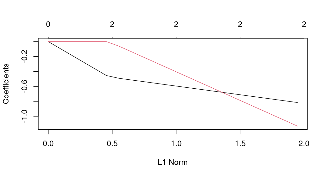
coef(fit1)## 3 x 56 sparse Matrix of class "dgCMatrix"
##
## (Intercept) 22.53281 23.60072190 24.5737668 25.4603691 26.2682081 27.0042808
## V1 . -0.08439977 -0.1613017 -0.2313719 -0.2952172 -0.3533907
## V2 . . . . . .
##
## (Intercept) 27.6749629 28.2860635 29.89390243 32.0395633 33.9946271 35.7760085
## V1 -0.4063962 -0.4546928 -0.49169909 -0.5208821 -0.5474709 -0.5716976
## V2 . . -0.06174822 -0.1580015 -0.2457061 -0.3256192
##
## (Intercept) 37.3991368 38.8780709 40.2256206 41.4534577 42.5722171 43.5915890
## V1 -0.5937720 -0.6138855 -0.6322121 -0.6489106 -0.6641256 -0.6779890
## V2 -0.3984331 -0.4647784 -0.5252297 -0.5803108 -0.6304985 -0.6762278
##
## (Intercept) 44.5204027 45.3667032 46.1378206 46.8404342 47.4805518 48.0638808
## V1 -0.6906209 -0.7021305 -0.7126176 -0.7221731 -0.7308874 -0.7388199
## V2 -0.7178946 -0.7558598 -0.7904523 -0.8219716 -0.8506815 -0.8768503
##
## (Intercept) 48.5953884 49.0796784 49.5209454 49.9230114 50.2893590 50.6231613
## V1 -0.7460477 -0.7526334 -0.7586340 -0.7641015 -0.7690833 -0.7736226
## V2 -0.9006943 -0.9224201 -0.9422158 -0.9602529 -0.9766877 -0.9916624
##
## (Intercept) 50.9273095 51.2044380 51.4569472 51.6870242 51.8966618 52.0876757
## V1 -0.7777586 -0.7815271 -0.7849609 -0.7880896 -0.7909404 -0.7935379
## V2 -1.0053069 -1.0177392 -1.0290670 -1.0393885 -1.0487931 -1.0573622
##
## (Intercept) 52.2617205 52.4203036 52.5647987 52.6964572 52.8164195 52.9257247
## V1 -0.7959047 -0.7980612 -0.8000262 -0.8018165 -0.8034479 -0.8049343
## V2 -1.0651700 -1.0722843 -1.0787665 -1.0846728 -1.0900545 -1.0949580
##
## (Intercept) 53.0253195 53.1159879 53.1986801 53.274026 53.342679 53.405233
## V1 -0.8062886 -0.8075304 -0.8086542 -0.809678 -0.810611 -0.811461
## V2 -1.0994259 -1.1034874 -1.1071976 -1.110578 -1.113658 -1.116465
##
## (Intercept) 53.4622294 53.5141626 53.5614822 53.6045981 53.6438837 53.6796793
## V1 -0.8122355 -0.8129413 -0.8135843 -0.8141702 -0.8147041 -0.8151905
## V2 -1.1190224 -1.1213525 -1.1234756 -1.1254101 -1.1271728 -1.1287789
##
## (Intercept) 53.7122949 53.7420130
## V1 -0.8156337 -0.8160375
## V2 -1.1302422 -1.1315756cvfit <- cv.glmnet(X, y)
plot(cvfit)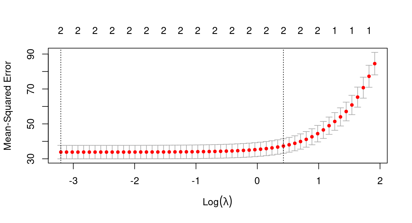
cvfit$lambda.min## [1] 0.04063097