Chapter 14 簡單線性迴歸分析二部曲

14.1 續

14.1.1 簡單線性迴歸分析首部曲的「續」

繼續往前走之前，作者小編一定要再一次提醒大家，本波士頓數據集案例分析微微書的總目標是

搜尋「1970年代波士頓都會區的最佳『hedonic housing price model』」，某一種迴歸模型。

接下來，我們繼續研究「兩個連續型變數的迴歸模型」，尤其是固定一個變數在「房價中位數」。「房價中位數」是我們「散佈圖」的「y變數」，其他連續型變數則是我們的「x變數」，而且一次只來、只看一個。沿著、順著這樣的「探索之路」，作者小編想在這一章好好解釋、分析、視覺化「簡單線性迴歸模型」。「簡單線性迴歸模型」是最簡單的「兩個連續型變數的迴歸模型」：

\[y = \beta_0 + \beta_1 x + \epsilon\]

接下來幾章，除了介紹「最小平方法(LS)」，也會介紹「LASSO」跟「Ridge」。進而介紹作者小編土耳其同學反對的「機器學習(ML)」。以上不論是

1. LS
2. LASSO
3. Ridge
4. ML
5. …

都是「挑選模型」的標準，或說是「估計模型」的演算法。「估計」兩個字對讀者諸君而言，或許太遙遠，但「估計」其實骨子裡就是「猜測」，不只是「有憑有據的猜測」，而且這些「猜測」都必須根據「樣本」。現實裡的「樣本」，讓「估計、猜測」的辦法不會只有一種，也就是說，現實裡沒有打遍天下無敵手的猜測辦法，意思是說「沒有贏家演算法」。即便如此，無論如何，接下來R將協助我們全掌握「簡單線性迴歸分析」，並且學習各種演算法的優缺點。

…

作者小編一路寫下來，感覺上，好像我們已經遠離了「分配」。事實上不然，因為「簡單線性迴歸模型」，「x變數」把「y變數的分配」切成許許多多的「小分配」。然後，統計學家企圖把這一些「小分配的平均數」連成「一條直線」：

\[E(y|x = x_0) = \beta_0 + \beta_1 x_0\]

只是不知道，\(\beta_0\)跟\(\beta_1\)到底在哪裡？到底有多大？而已。接下來，我們將好好想辦法

發展

找到\(\beta_0\)跟\(\beta_1\)的辦法、技術、數學、…，任何科學的辦法。

…

14.1.2 繼續的「續」

這一章將繼續談「最小平方法」。上一章，作者小編談過

1. 引用知名數據集「anscombe」示範「散佈圖」的重要性、
2. 什麼是「最小平方法」？
3. 引用「相關係數」挑「簡單線性迴歸線」的「解釋變數」、
4. 變數變換如何影響「簡單線性迴歸線」的「解釋能力」、
5. 取得「最小平方法迴歸線」的報表、
6. 抓取報表內的各種數字、

接著，我們將討論

1. 最小平方法「lsfit」家族的其他成員，「ls.print」跟「ls.diag」、
2. 什麼是「迴歸診斷」？
3. 深入探討知名數據集「anscombe」的第二組、第三組跟第四組子數據集、
4. 介紹最簡單的「非線性迴歸線」、
5. 示範各種波士頓數據集「房價中位數」與「低社經人口比例」的「非線性迴歸線」、

作者小編持續努力為大家「『示範』『程式能力』的重要性」。

14.2 學習目標

14.3 準備工作

「學習」其實是「找答案之旅」。

如果沒有問題，作者小編認為「不一定要學習」。但是，作者小編認為

為個人增添「光」與「彩」也是一種問題(『How』跟『Why』的問題)，

所以嚴格說起來，「學習」是一條「必經之路」。為此，作者小編在這一整套微微書總是「不厭其煩」地出現「昔日在前面章節出現過的程式碼」，還請讀者諸君見諒！

14.3.1 波士頓數據集

require(MASS) # 用「require」不用「library」，是因為如果R已經將套件MASS載入環境，就不需要再載一次。
data(Boston)
boston <- Boston 
# 「不動」原始數據集，不論它有「多原始」，是R程式設計的一項絕佳習慣。
# 即便一般使用者是無法任意改變套件MASS的內容物！
### rad (index of accessibility to radial highways)
boston[,"rad"] <- factor(boston[,"rad"], ordered = TRUE)
### chas (= 1 if tract bounds river; 0 otherwise)
boston[,"chas"] <- factor(boston[,"chas"])
head(boston)

##      crim zn indus chas   nox    rm  age    dis rad tax ptratio  black lstat
## 1 0.00632 18  2.31    0 0.538 6.575 65.2 4.0900   1 296    15.3 396.90  4.98
## 2 0.02731  0  7.07    0 0.469 6.421 78.9 4.9671   2 242    17.8 396.90  9.14
## 3 0.02729  0  7.07    0 0.469 7.185 61.1 4.9671   2 242    17.8 392.83  4.03
## 4 0.03237  0  2.18    0 0.458 6.998 45.8 6.0622   3 222    18.7 394.63  2.94
## 5 0.06905  0  2.18    0 0.458 7.147 54.2 6.0622   3 222    18.7 396.90  5.33
## 6 0.02985  0  2.18    0 0.458 6.430 58.7 6.0622   3 222    18.7 394.12  5.21
##   medv
## 1 24.0
## 2 21.6
## 3 34.7
## 4 33.4
## 5 36.2
## 6 28.7

tail(boston)

##        crim zn indus chas   nox    rm  age    dis rad tax ptratio  black lstat
## 501 0.22438  0  9.69    0 0.585 6.027 79.7 2.4982   6 391    19.2 396.90 14.33
## 502 0.06263  0 11.93    0 0.573 6.593 69.1 2.4786   1 273    21.0 391.99  9.67
## 503 0.04527  0 11.93    0 0.573 6.120 76.7 2.2875   1 273    21.0 396.90  9.08
## 504 0.06076  0 11.93    0 0.573 6.976 91.0 2.1675   1 273    21.0 396.90  5.64
## 505 0.10959  0 11.93    0 0.573 6.794 89.3 2.3889   1 273    21.0 393.45  6.48
## 506 0.04741  0 11.93    0 0.573 6.030 80.8 2.5050   1 273    21.0 396.90  7.88
##     medv
## 501 16.8
## 502 22.4
## 503 20.6
## 504 23.9
## 505 22.0
## 506 11.9

### 讀取自製的波士頓數據集中文資訊。
DISvars <- colnames(boston)[which(sapply(boston, class) == "integer")]
CONvars <- colnames(boston)[which(sapply(boston, class) == "numeric")]
colsBostonFull<-readRDS("output/data/colsBostonFull.rds")
colsBostonFull$內容物 <- sapply(boston, class)
colsBostonFull

##     變數名
## 1     crim
## 2       zn
## 3    indus
## 4     chas
## 5      nox
## 6       rm
## 7      age
## 8      dis
## 9      rad
## 10     tax
## 11 ptratio
## 12   black
## 13   lstat
## 14    medv
##                                                                     說明
## 1                                          per capita crime rate by town
## 2       proportion of residential land zoned for lots over 25,000 sq.ft.
## 3                       proportion of non-retail business acres per town
## 4  Charles River dummy variable (= 1 if tract bounds river; 0 otherwise)
## 5                     nitric oxides concentration (parts per 10 million)
## 6                                   average number of rooms per dwelling
## 7                 proportion of owner-occupied units built prior to 1940
## 8                   weighted distances to five Boston employment centres
## 9                              index of accessibility to radial highways
## 10                              full-value property-tax rate per $10,000
## 11                                           pupil-teacher ratio by town
## 12        1000(Bk - 0.63)^2 where Bk is the proportion of blacks by town
## 13                                      % lower status of the population
## 14                       Median value of owner-occupied homes in $1000's
##                            中文翻譯   中文變數名稱          內容物
## 1              每個城鎮人均犯罪率。         犯罪率         numeric
## 2  超過25,000平方呎的住宅用地比例。   住宅用地比例         numeric
## 3    每個城鎮非零售業務英畝的比例。   非商業區比例         numeric
## 4           是否鄰近Charles River。         河邊宅          factor
## 5                  氮氧化合物濃度。       空汙指標         numeric
## 6            每個住宅的平均房間數。     平均房間數         numeric
## 7    1940年之前建造的自用住宅比例。     老房子比例         numeric
## 8  距波士頓五大商圈的加權平均距離。   加權平均距離         numeric
## 9          環狀高速公路的可觸指標。     交通便利性 ordered, factor
## 10         財產稅占比(每一萬美元)。       財產稅率         numeric
## 11                         生師比。         生師比         numeric
## 12                     黑人的比例。       黑人指數         numeric
## 13     (比較)低社經地位人口的比例。 低社經人口比例         numeric
## 14         以千美元計的房價中位數。     房價中位數         numeric

14.3.2 anscombe數據集

這一組Tufte教授在「The Visual Display of Quantitative Information」這本書的第十頁用來示範「散佈圖」的數據集，源自於

Anscombe, Francis J. (1973). Graphs in statistical analysis. The American Statistician, 27, 17–21.

anscombe這一個字，在統計界已經是「幾乎一樣的平均數、標準差加相關係數卻完全不一樣的兩維數據集」的「代名詞」了！後來又有兩位學者「Justin Matejka」跟「George Fitzmaurice」循著同樣的思路，利用「Simulated Annealing」演算法找到「比anscombe更anscombe」的數據集，

datasauRus::datasauRus

作者小編企圖在這裡「深入挖掘」這兩大組數據集可能隱藏的「教學契機」。請讀者諸君不要轉台！

require(datasets) # 通常我們是這麼寫「library(datasets)」。
data("anscombe") # 載入。

14.3.3 datasauRus::datasaurus_dozen數據集

require(datasauRus) # 通常我們是這麼寫「library(datasauRus)」。
data(datasaurus_dozen) # 載入。

14.4 回顧最小平方法

在上一章，作者小編這麼示範「最小平方法」：

「最小平方法迴歸線」在幾何上，就是「按著那顆『黑點』轉動『直線』直到『SSE』出現最小為止」，得到的那一條直線就是答案，就是「最小平方法迴歸線」。

請看作者小編示範這個想法、理論、演算法：

• (動作一：準備動作)準備數據，加上計算單變量與雙變量的摘要統計量。

df <- anscombe[, c("x1", "y1")] # 取出「x1」跟「y1」，其中「1」代表第一組。
colnames(df) <- c("x", "y") # 劃掉其中的「1」。
df # 呼叫出來再一次檢視這一組數據集。

##     x     y
## 1  10  8.04
## 2   8  6.95
## 3  13  7.58
## 4   9  8.81
## 5  11  8.33
## 6  14  9.96
## 7   6  7.24
## 8   4  4.26
## 9  12 10.84
## 10  7  4.82
## 11  5  5.68

summary(df) # 單變量的摘要統計量。

##        x              y         
##  Min.   : 4.0   Min.   : 4.260  
##  1st Qu.: 6.5   1st Qu.: 6.315  
##  Median : 9.0   Median : 7.580  
##  Mean   : 9.0   Mean   : 7.501  
##  3rd Qu.:11.5   3rd Qu.: 8.570  
##  Max.   :14.0   Max.   :10.840

cor(df) # 雙變量的摘要統計量。

##           x         y
## x 1.0000000 0.8164205
## y 0.8164205 1.0000000

# 繪製散佈圖。左右上下各加3個單位，方便大家觀察。
plot(df, 
     xlim = range(df[, "x"]) + c(-3, 3),
     ylim = range(df[, "y"]) + c(-3, 3))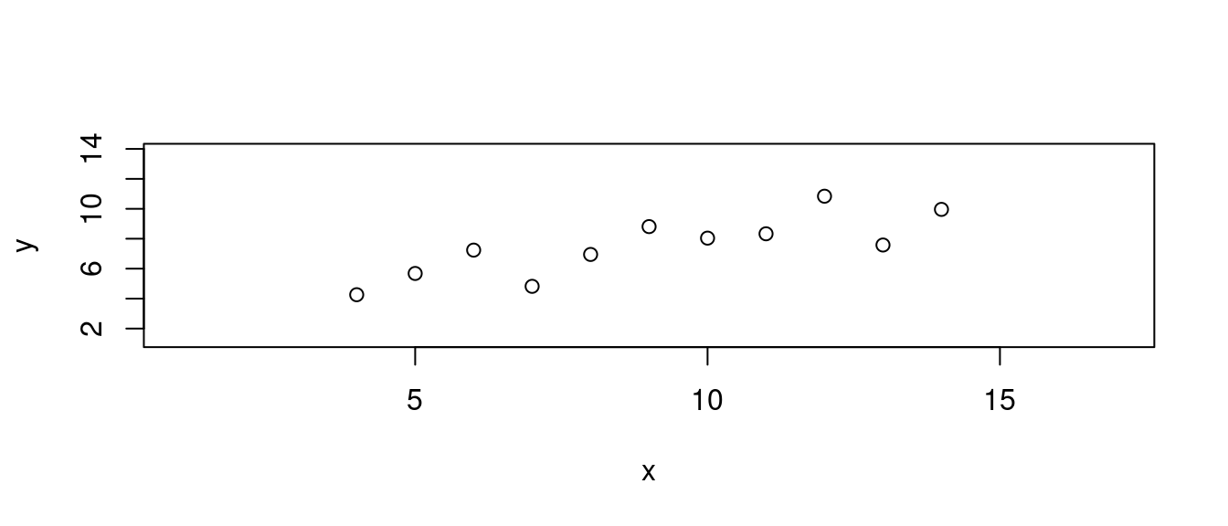

• (動作二：搜尋最小平方法迴歸線)呼叫最小平方法R的函式「lsfit」。

###
m1 <- lsfit(df[c(1,2,3,4,5,6,7,8,9,10,11), "x"], df[c(1,2,3,4,5,6,7,8,9,10,11), "y"])
m1$coefficients

## Intercept         X 
## 3.0000909 0.5000909

• (動作三：再一次搜尋最小平方法迴歸線)現在，只有「一個x」加「一個y」，那「最小平方法迴歸線」在幾何上，就是「按著那顆『黑點』轉動『直線』直到『\(SSE\)』出現最小值為止」，得到的那一條直線就是答案，就是「最小平方法迴歸線」。

###
SSE <- numeric(0) # 準備放置各種可能直線的SSE。
ybar <- mean(df[, "y"]) # 全部y座標的平均數。
xbar <- mean(df[, "x"]) # 全部x座標的平均數。
for (b in seq(-1, 1, 0.1)) {
  a <- ybar - b * xbar
  predy <- df[, "y"] - (a + b * df[, "x"])
  SSE <- c(SSE, sum(predy^2))
} 
# 透過觀察散佈圖，或是計算幾組點對點的斜率，定調「斜率」可能的範圍。
# 加上「最小平方法迴歸線」一定通過(xbar,ybar)這一點，就可以取得對應某一個斜率的「截距」。
plot(seq(-1, 1, 0.1), SSE, type = "l") # 顯示SSE的搜尋成果。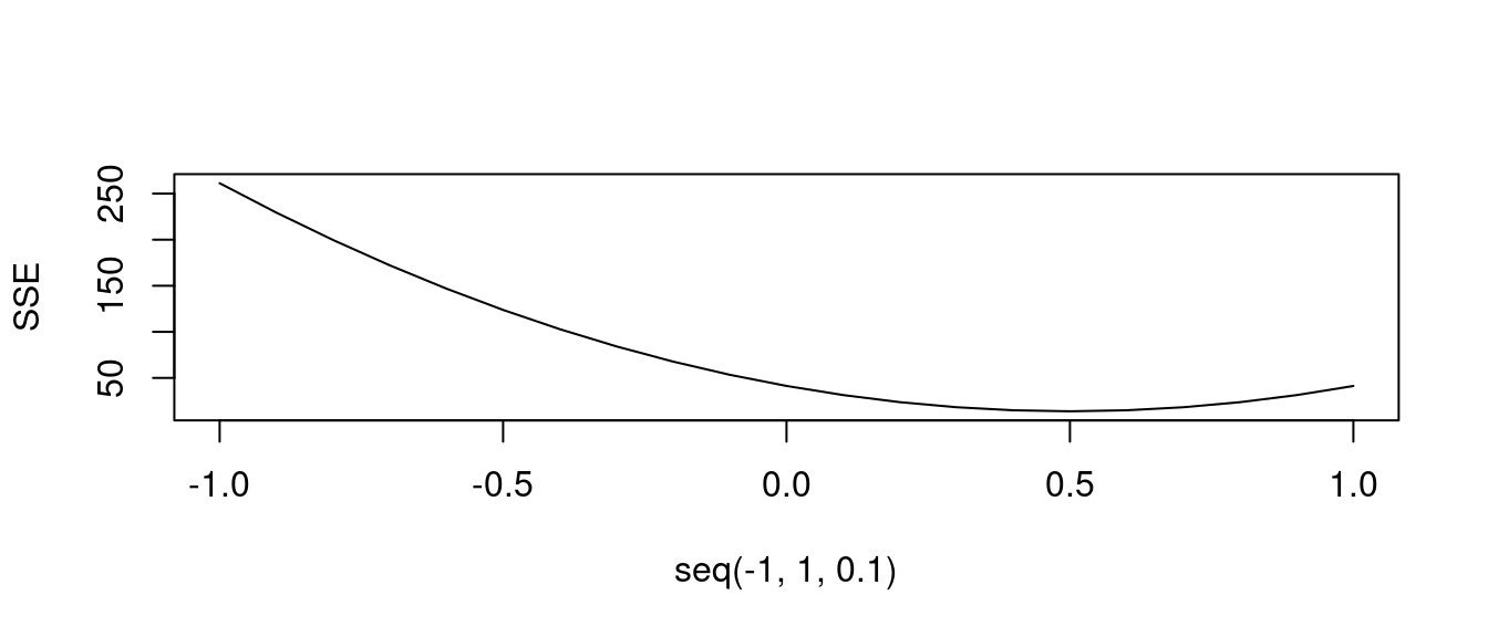

b <- seq(-1, 1, 0.1)[which.min(SSE)] # 最小化SSE的斜率等於多少？
a <- ybar - b * xbar # 對應上述斜率的截距。
LINE <- c(a, b)
names(LINE) <- c("a", "b")
LINE # 報告成果。

##        a        b 
## 3.000909 0.500000

• (動作四：驗證作者小編的理論)結論：答案是一樣的！也就是說，作者小編的理論得到證實。

plot(df[, c("x", "y")], 
     xlim = range(df[, "x"]) + c(-3, 3),
     ylim = range(df[, "y"]) + c(-3, 3)) # 最簡散佈圖。
abline(a = LINE["a"], b = LINE["b"], col = "red", lwd = 8) # 畫上搜尋成果的直線。
abline(m1, lwd = 3, col = "green") # 畫上R提供的答案直線。
title(paste0("迴圈搜尋成果：", "y = ", 
             round(LINE["a"], 2), 
             " + ", round(LINE["b"], 2), "x", 
             "; R提供的成果：", 
             "y = ", 
             round(m1$coefficients[1], 2), 
             " + ", round(m1$coefficients[2], 2), "x"))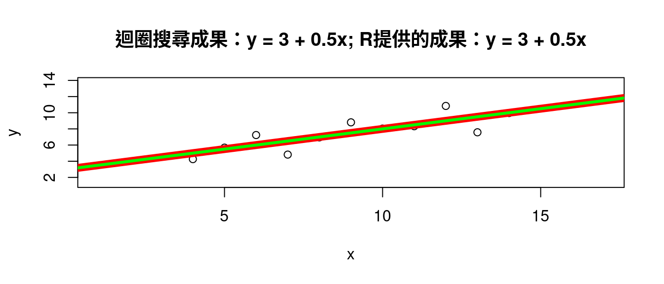

…

14.5 最小平方法的二部曲

整個發展已經進入第六章了，作者小編好像進入了「腸枯思竭」的狀態了。遇上這種「時候」，作者小編會「停下來翻書，找答案、找靈感」。

停在哪裡，就從哪裡找書、翻書？

所以，在回顧作者小編前一章的程式碼之前，讓我們先檢視「好幾下」最小平方法(lsfit)的R官方使用手冊：

knitr::include_url("https://www.rdocumentation.org/packages/stats/versions/3.6.2/topics/lsfit")

作者小編到目前為止，未曾討論過

如何『使用』使用手冊？

幾個重點：

1. (重點一)先仔細閱讀「簡介」，簡介「只是」一段言簡意賅的英文。比如說，「lsfit」的簡介就是

Find The Least Squares Fit

The least squares estimate of in the model \(\bold Y = \bold X \beta + \bold \epsilon\) is found.

第一段讓我們知道「lsfit」這個「名字」是怎麼來的？接下來，「lsfit作者介紹『lsfit』的主要功能」。

2. (重點二)剪貼範例到自己的環境，並進行測試。比如說，這兩句話就是「lsfit作者」提供的範例：

lsD9 <- lsfit(x = unclass(gl(2, 10)), y = weight)
ls.print(lsD9)

3. (重點三)在「See Also」這一段，「手冊作者」會建議「同時參考的手冊」。比如說，「lsfit作者」建議了「lm」、「ls.print」、「ls.diag」。

…

作者小編原本安排在這一章討論「LASSO」跟「Ridge」，只根據個人看過「符號」之後對這兩種演算法的想像，但經過測試，發現事實不然，「LASSO」跟「Ridge」無法用在「簡單線性迴歸建模」。作者小編心想「慘了」。好消息是

2021/02/08的早上看過一本談論「深度學習(Deep Learning)」的書，提到「挖掘結構的演算法」；

同一天，驚覺尚未討論「迴歸建模的第三階段：迴歸診斷」，在前一章，作者小編只顯示一張表跟幾張圖，完全沒解釋「什麼是迴歸診斷」。同時也瀏覽了「ls.diag」的「Value」橋段。…

基於這兩點，作者小編找到了這一章的題材！！！

…

嚴格說起來，作者小編在上一章完全倚重「lm」為大家解析「如何搜尋最小平方法迴歸線」。雖然，官方使用手冊也是這麼建議

lm which usually is preferable;

但是，「lsfit」家族的另外兩位成員：「ls.print」跟「ls.diag」完整呈現「如何搜尋最小平方法迴歸線」的三部曲：

1. 找線
2. 列印
3. 診斷

### 找線
m1 <- lsfit(df[, "x"], df[, "y"])
### 列印
ls.print(m1)

## Residual Standard Error=1.2366
## R-Square=0.6665
## F-statistic (df=1, 9)=17.9899
## p-value=0.0022
## 
##           Estimate Std.Err t-value Pr(>|t|)
## Intercept   3.0001  1.1247  2.6673   0.0257
## X           0.5001  0.1179  4.2415   0.0022

### 診斷
ls.diag(m1)

## $std.dev
## [1] 1.236603
## 
## $hat
##  [1] 0.10000000 0.10000000 0.23636364 0.09090909 0.12727273 0.31818182
##  [7] 0.17272727 0.31818182 0.17272727 0.12727273 0.23636364
## 
## $std.res
##  [1]  0.03324397 -0.04331791 -1.77793266  1.11028824 -0.14810075 -0.04050923
##  [7]  1.10190458 -0.72515977  1.63487302 -1.45488131  0.16606601
## 
## $stud.res
##  [1]  0.03134464 -0.04084477 -2.08109891  1.12679993 -0.13980118 -0.03819595
##  [7]  1.11695887 -0.70458079  1.83833042 -1.56846043  0.15680897
## 
## $cooks
##  [1] 0.00006139788 0.00010424672 0.48920927577 0.06163699895 0.00159934188
##  [6] 0.00038289951 0.12675648475 0.12269989634 0.27902959338 0.15434122237
## [11] 0.00426801143
## 
## $dfits
##  [1]  0.01044821 -0.01361492 -1.15781655  0.35632543 -0.05338746 -0.02609280
##  [7]  0.51037958 -0.48132031  0.84000076 -0.59896572  0.08724046
## 
## $correlation
##            Intercept          X
## Intercept  1.0000000 -0.9434564
## X         -0.9434564  1.0000000
## 
## $std.err
##                [,1]
## Intercept 1.1247468
## X         0.1179055
## 
## $cov.scaled
##            Intercept           X
## Intercept  1.2650553 -0.12511536
## X         -0.1251154  0.01390171
## 
## $cov.unscaled
##             Intercept            X
## Intercept  0.82727273 -0.081818182
## X         -0.08181818  0.009090909

14.5.1 把ls.print的輸出統計量收錄在一張表

x <- sapply(1, function(w){
  ls.print(m1)
})

## Residual Standard Error=1.2366
## R-Square=0.6665
## F-statistic (df=1, 9)=17.9899
## p-value=0.0022
## 
##           Estimate Std.Err t-value Pr(>|t|)
## Intercept   3.0001  1.1247  2.6673   0.0257
## X           0.5001  0.1179  4.2415   0.0022

x

##            [,1]       
## summary    character,6
## coef.table list,1

x["summary",1]

## $summary
##      Mean Sum Sq R Squared F-value   Df 1 Df 2 Pr(>F)  
## [1,] "1.2366"    "0.6665"  "17.9899" "1"  "9"  "0.0022"

x["summary",1]$summary

##      Mean Sum Sq R Squared F-value   Df 1 Df 2 Pr(>F)  
## [1,] "1.2366"    "0.6665"  "17.9899" "1"  "9"  "0.0022"

x["coef.table",1]

## $coef.table
## $coef.table[[1]]
##            Estimate   Std.Err  t-value    Pr(>|t|)
## Intercept 3.0000909 1.1247468 2.667348 0.025734051
## X         0.5000909 0.1179055 4.241455 0.002169629

x["coef.table",1]$coef.table

## [[1]]
##            Estimate   Std.Err  t-value    Pr(>|t|)
## Intercept 3.0000909 1.1247468 2.667348 0.025734051
## X         0.5000909 0.1179055 4.241455 0.002169629

x["coef.table",1]$coef.table[[1]]

##            Estimate   Std.Err  t-value    Pr(>|t|)
## Intercept 3.0000909 1.1247468 2.667348 0.025734051
## X         0.5000909 0.1179055 4.241455 0.002169629

檢查過後，

LSsum <- x["summary",1]$summary
class(LSsum)

## [1] "matrix" "array"

LScoef <- x["coef.table",1]$coef.table[[1]]
class(LScoef)

## [1] "matrix" "array"

14.5.2 把ls.diag的輸出統計量收錄在一張表

x <- sapply(1, function(w){
  ls.diag(m1)
})
x

##              [,1]      
## std.dev      1.236603  
## hat          numeric,11
## std.res      numeric,11
## stud.res     numeric,11
## cooks        numeric,11
## dfits        numeric,11
## correlation  numeric,4 
## std.err      numeric,2 
## cov.scaled   numeric,4 
## cov.unscaled numeric,4

14.5.2.1 關於迴歸係數的摘要統計量

x["std.err",1]

## $std.err
##                [,1]
## Intercept 1.1247468
## X         0.1179055

x["std.err",1]$std.err

##                [,1]
## Intercept 1.1247468
## X         0.1179055

class(x["std.err",1]$std.err)

## [1] "matrix" "array"

x["std.err",1]$std.err["Intercept",1]

## Intercept 
##  1.124747

x["std.err",1]$std.err["X",1]

##         X 
## 0.1179055

x["correlation",1]

## $correlation
##            Intercept          X
## Intercept  1.0000000 -0.9434564
## X         -0.9434564  1.0000000

x["correlation",1]$correlation

##            Intercept          X
## Intercept  1.0000000 -0.9434564
## X         -0.9434564  1.0000000

class(x["correlation",1]$correlation)

## [1] "matrix" "array"

x["correlation",1]$correlation["Intercept", "X"]

## [1] -0.9434564

14.5.2.1.1 課堂練習

1. 抓「cov.scaled」
2. 抓「cov.unscaled」

14.5.2.2 關於戴帽子y的摘要統計量

x["hat",1]$hat

##  [1] 0.10000000 0.10000000 0.23636364 0.09090909 0.12727273 0.31818182
##  [7] 0.17272727 0.31818182 0.17272727 0.12727273 0.23636364

x["std.res",1]$std.res

##  [1]  0.03324397 -0.04331791 -1.77793266  1.11028824 -0.14810075 -0.04050923
##  [7]  1.10190458 -0.72515977  1.63487302 -1.45488131  0.16606601

x["stud.res",1]$stud.res

##  [1]  0.03134464 -0.04084477 -2.08109891  1.12679993 -0.13980118 -0.03819595
##  [7]  1.11695887 -0.70458079  1.83833042 -1.56846043  0.15680897

x["cooks",1]$cooks

##  [1] 0.00006139788 0.00010424672 0.48920927577 0.06163699895 0.00159934188
##  [6] 0.00038289951 0.12675648475 0.12269989634 0.27902959338 0.15434122237
## [11] 0.00426801143

x["dfits",1]$dfits

##  [1]  0.01044821 -0.01361492 -1.15781655  0.35632543 -0.05338746 -0.02609280
##  [7]  0.51037958 -0.48132031  0.84000076 -0.59896572  0.08724046

14.5.2.3 關於誤差的摘要統計量

x["std.dev",1]$std.dev

## [1] 1.236603

14.5.3 請專家幫忙

m1 <- lm(y ~ x, data = df)
require(broom)
tidy(m1)

## # A tibble: 2 × 5
##   term        estimate std.error statistic p.value
##   <chr>          <dbl>     <dbl>     <dbl>   <dbl>
## 1 (Intercept)    3.00      1.12       2.67 0.0257 
## 2 x              0.500     0.118      4.24 0.00217

augment(m1)

## # A tibble: 11 × 8
##        y     x .fitted  .resid   .hat .sigma   .cooksd .std.resid
##    <dbl> <dbl>   <dbl>   <dbl>  <dbl>  <dbl>     <dbl>      <dbl>
##  1  8.04    10    8.00  0.0390 0.100    1.31 0.0000614     0.0332
##  2  6.95     8    7.00 -0.0508 0.1      1.31 0.000104     -0.0433
##  3  7.58    13    9.50 -1.92   0.236    1.06 0.489        -1.78  
##  4  8.81     9    7.50  1.31   0.0909   1.22 0.0616        1.11  
##  5  8.33    11    8.50 -0.171  0.127    1.31 0.00160      -0.148 
##  6  9.96    14   10.0  -0.0414 0.318    1.31 0.000383     -0.0405
##  7  7.24     6    6.00  1.24   0.173    1.22 0.127         1.10  
##  8  4.26     4    5.00 -0.740  0.318    1.27 0.123        -0.725 
##  9 10.8     12    9.00  1.84   0.173    1.10 0.279         1.63  
## 10  4.82     7    6.50 -1.68   0.127    1.15 0.154        -1.45  
## 11  5.68     5    5.50  0.179  0.236    1.31 0.00427       0.166

glance(m1)

## # A tibble: 1 × 12
##   r.squared adj.r.squared sigma statistic p.value    df logLik   AIC   BIC
##       <dbl>         <dbl> <dbl>     <dbl>   <dbl> <dbl>  <dbl> <dbl> <dbl>
## 1     0.667         0.629  1.24      18.0 0.00217     1  -16.8  39.7  40.9
## # ℹ 3 more variables: deviance <dbl>, df.residual <int>, nobs <int>

14.6 迴歸建模的第三階段：迴歸診斷

14.6.1 什麼是殘差？

14.6.2 殘差的變形

14.6.3 殘差的函數

14.7 迴歸診斷當x變數是低社經人口比例時的最小平方法迴歸線

CORmedv <- cor(x = boston[, CONvars[-12]], y = boston[, "medv"])
maxCOR <- rownames(CORmedv)[which.max(abs(CORmedv[,1]))]
plot(boston[, maxCOR], boston[, "medv"], 
     xlab = colsBostonFull$中文變數名稱[which(colsBostonFull$變數名 == maxCOR)],
     ylab = "房價中位數")
title(paste0("最高相關係數", " = ", 
             cor(boston[, maxCOR], 
                 boston[, "medv"])))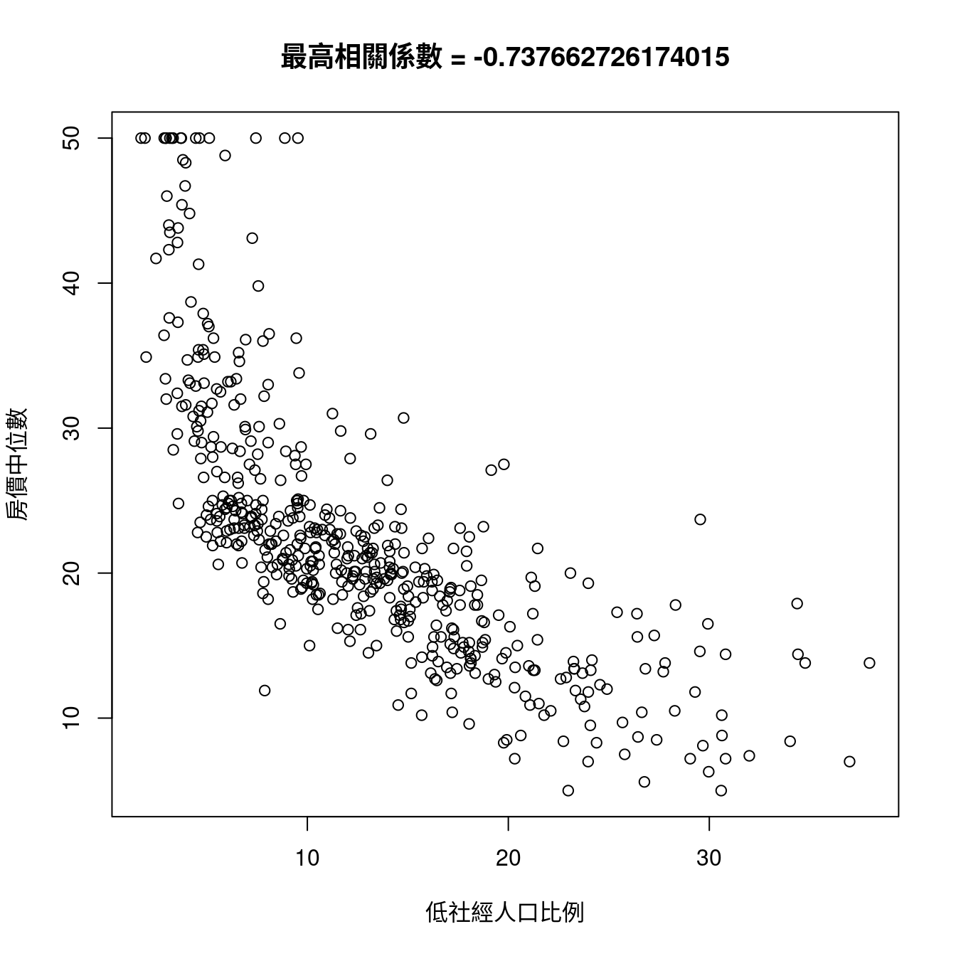

m1 <- lm(medv ~ lstat, data = boston)
par(mfrow = c(2, 2))
plot(m1)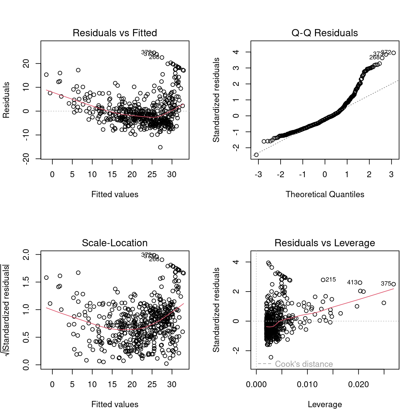

boston$lstat10 <- boston$lstat^(1/10)
m0 <- lm(medv ~ lstat10, data = boston)
par(mfrow = c(2, 2))
plot(m0)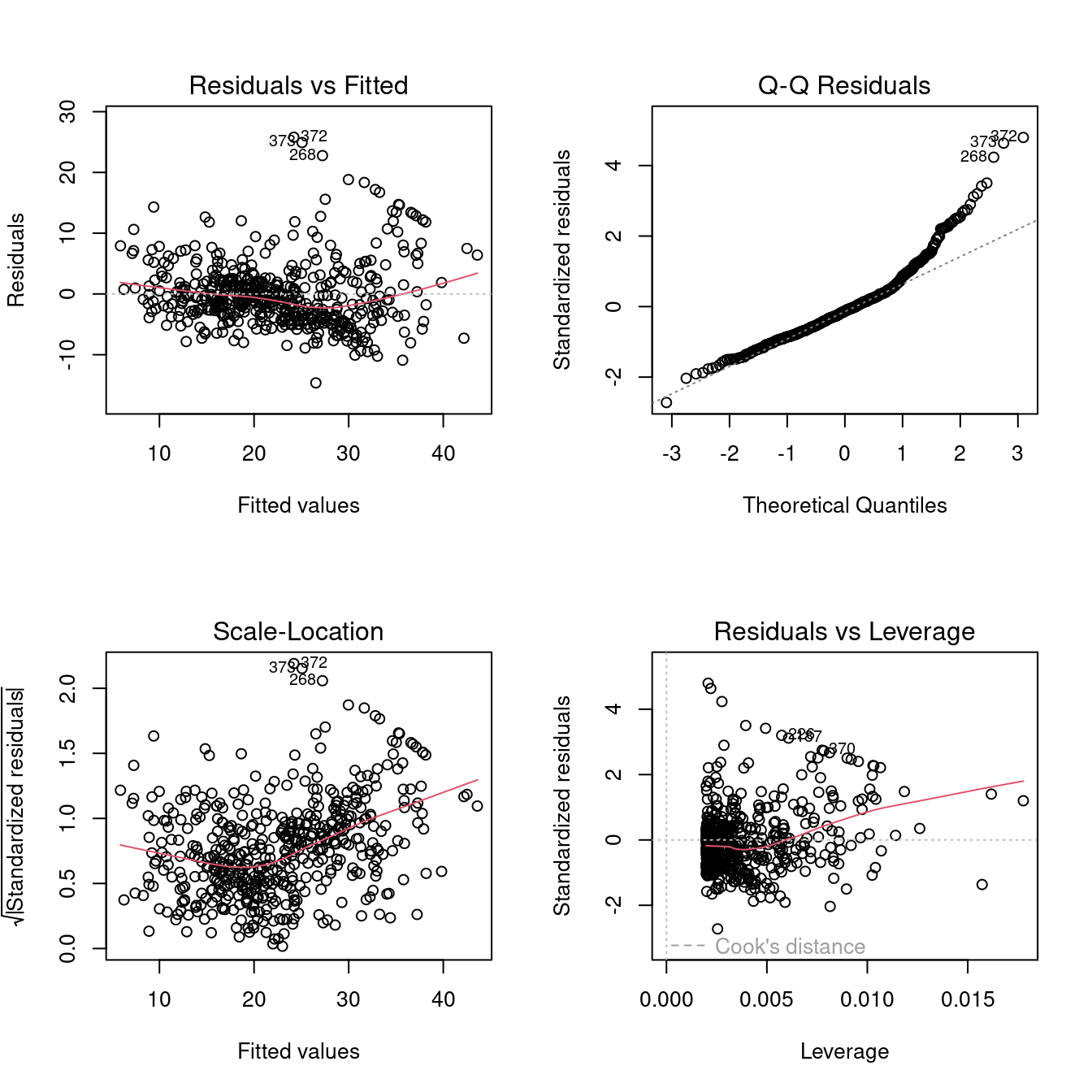

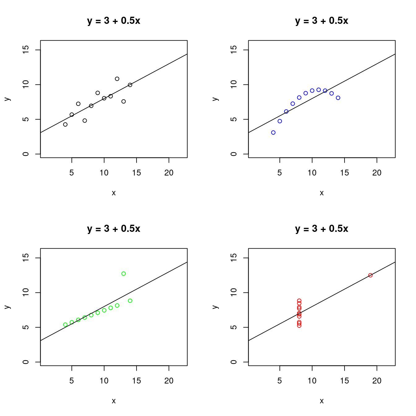
14.8 繼續挖Anscombe數據集

全部子數據集的散佈圖：

14.8.1 繼續挖Anscombe數據集之「y3」

寫一支程式找到y = 4.01 + 0.35x。

14.8.2 繼續挖Anscombe數據集之「y2」

Q1: 找到曲線方程式的估計？

df <- anscombe[, c("x2", "y2")] # 取出「x1」跟「y1」，其中「1」代表第一組。
colnames(df) <- c("x", "y") # 劃掉其中的「1」。
df # 呼叫出來再一次檢視這一組數據集。

##     x    y
## 1  10 9.14
## 2   8 8.14
## 3  13 8.74
## 4   9 8.77
## 5  11 9.26
## 6  14 8.10
## 7   6 6.13
## 8   4 3.10
## 9  12 9.13
## 10  7 7.26
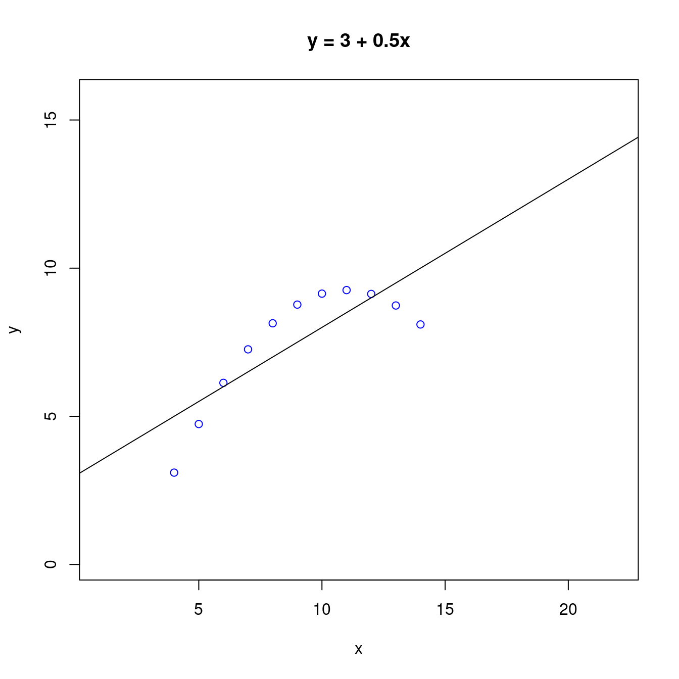
## 11  5 4.74

# 繪製散佈圖。左右上下各加3個單位，方便大家觀察。
plot(df, 
     xlim = range(df[, "x"]) + c(-3, 3),
     ylim = range(df[, "y"]) + c(-3, 3))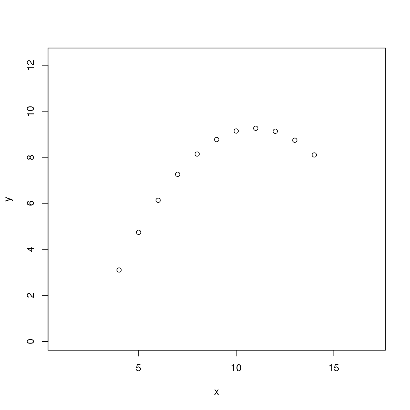

m2poly <- lm(y ~ poly(x, 2, raw = TRUE), data = df)
m2poly

## 
## Call:
## lm(formula = y ~ poly(x, 2, raw = TRUE), data = df)
## 
## Coefficients:
##             (Intercept)  poly(x, 2, raw = TRUE)1  poly(x, 2, raw = TRUE)2  
##                 -5.9957                   2.7808                  -0.1267

summary(m2poly)

## 
## Call:
## lm(formula = y ~ poly(x, 2, raw = TRUE), data = df)
## 
## Residuals:
##        Min         1Q     Median         3Q        Max 
## -0.0013287 -0.0011888 -0.0006294  0.0008741  0.0023776 
## 
## Coefficients:
##                           Estimate Std. Error t value            Pr(>|t|)    
## (Intercept)             -5.9957343  0.0043299   -1385 <0.0000000000000002 ***
## poly(x, 2, raw = TRUE)1  2.7808392  0.0010401    2674 <0.0000000000000002 ***
## poly(x, 2, raw = TRUE)2 -0.1267133  0.0000571   -2219 <0.0000000000000002 ***
## ---
## Signif. codes:  0 '***' 0.001 '**' 0.01 '*' 0.05 '.' 0.1 ' ' 1
## 
## Residual standard error: 0.001672 on 8 degrees of freedom
## Multiple R-squared:      1,  Adjusted R-squared:      1 
## F-statistic: 7.378e+06 on 2 and 8 DF,  p-value: < 0.00000000000000022

summary(m2poly)$coefficients

##                           Estimate    Std. Error   t value
## (Intercept)             -5.9957343 0.00432994585 -1384.713
## poly(x, 2, raw = TRUE)1  2.7808392 0.00104005552  2673.741
## poly(x, 2, raw = TRUE)2 -0.1267133 0.00005709766 -2219.238
##                                                  Pr(>|t|)
## (Intercept)             0.0000000000000000000000828575731
## poly(x, 2, raw = TRUE)1 0.0000000000000000000000004288066
## poly(x, 2, raw = TRUE)2 0.0000000000000000000000019036403

fx <- function(x){
  A <- summary(m2poly)$coefficients[1]
  B <- summary(m2poly)$coefficients[2]
  C <- summary(m2poly)$coefficients[3]
  return(A + B * x + C * x^2)
}
curve(fx, from = min(df$x), to = max(df$x))
A <- summary(m2poly)$coefficients[1]
B <- summary(m2poly)$coefficients[2]
C <- summary(m2poly)$coefficients[3]
fx <- A + B * df$x + C * df$x^2
points(df$x, df$y)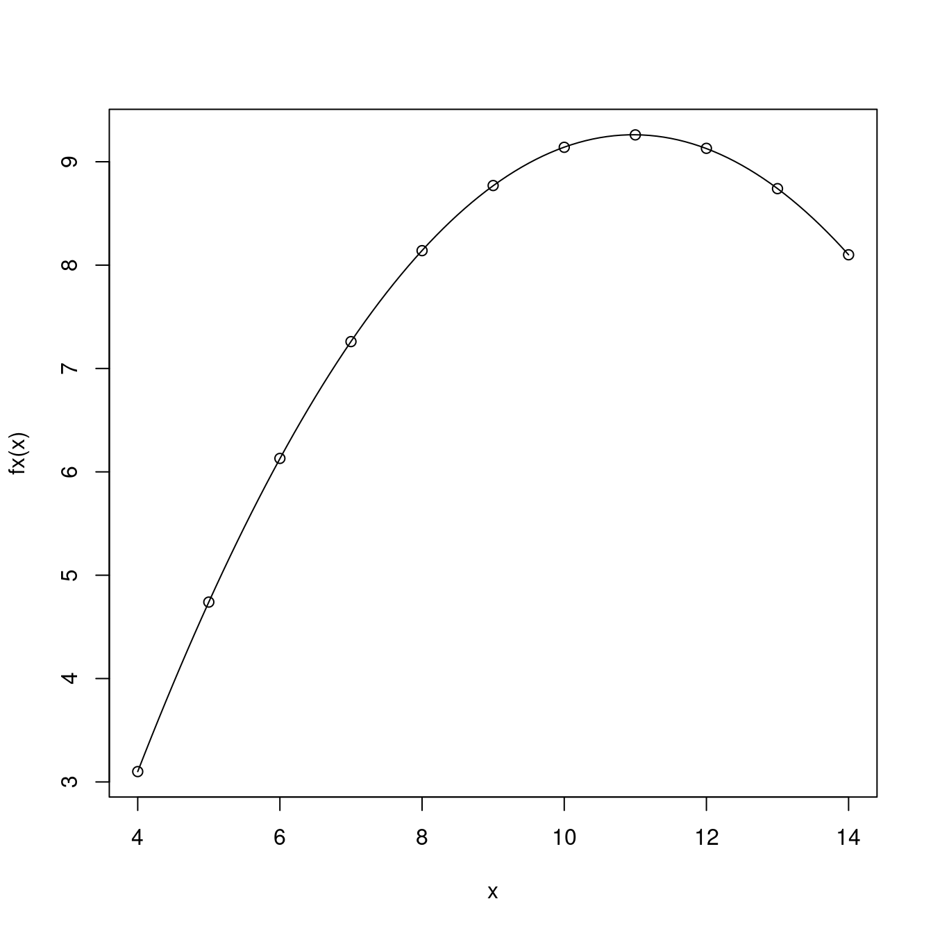

Q2: 找到曲線方程式的斜率方程式的估計？

fx <- expression(A + B * x + C * x^2)
D(fx,'x')

## B + C * (2 * x)

A <- summary(m2poly)$coefficients[1]
B <- summary(m2poly)$coefficients[2]
C <- summary(m2poly)$coefficients[3]
x <- df$x
eval(D(fx,'x'))

##  [1]  0.246573427  0.753426573 -0.513706294  0.500000000 -0.006853147
##  [6] -0.767132867  1.260279720  1.767132867 -0.260279720  1.006853147
## [11]  1.513706294

df$dy <- eval(D(fx,'x'))
m2D <- lm(dy ~ x, data = df)
m2D

## 
## Call:
## lm(formula = dy ~ x, data = df)
## 
## Coefficients:
## (Intercept)            x  
##      2.7808      -0.2534

summary(m2D)

## 
## Call:
## lm(formula = dy ~ x, data = df)
## 
## Residuals:
##                     Min                      1Q                  Median 
## -0.00000000000000024150 -0.00000000000000013165 -0.00000000000000007581 
##                      3Q                     Max 
##  0.00000000000000006650  0.00000000000000067134 
## 
## Coefficients:
##                            Estimate              Std. Error           t value
## (Intercept)  2.78083916083916182771  0.00000000000000024412 11391458854002518
## x           -0.25342657342657343156  0.00000000000000002559 -9903217624018514
##                        Pr(>|t|)    
## (Intercept) <0.0000000000000002 ***
## x           <0.0000000000000002 ***
## ---
## Signif. codes:  0 '***' 0.001 '**' 0.01 '*' 0.05 '.' 0.1 ' ' 1
## 
## Residual standard error: 0.0000000000000002684 on 9 degrees of freedom
## Multiple R-squared:      1,  Adjusted R-squared:      1 
## F-statistic: 9.807e+31 on 1 and 9 DF,  p-value: < 0.00000000000000022

plot(dy ~ x, data = df)
abline(m2D)

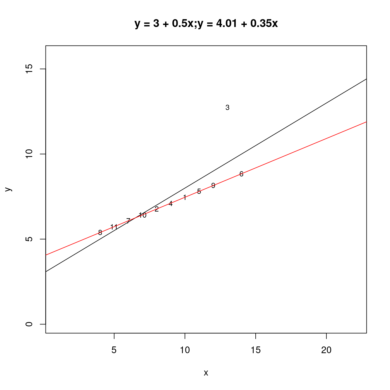
14.8.3 繼續挖Anscombe數據集之「y4」

m48 <- lm(y4[-8] ~ x4[-8], data = anscombe)
m48

## 
## Call:
## lm(formula = y4[-8] ~ x4[-8], data = anscombe)
## 
## Coefficients:
## (Intercept)       x4[-8]  
##       7.001           NA

summary(m48)

## 
## Call:
## lm(formula = y4[-8] ~ x4[-8], data = anscombe)
## 
## Residuals:
##    Min     1Q Median     3Q    Max 
## -1.751 -1.036 -0.036  0.859  1.839 
## 
## Coefficients: (1 not defined because of singularities)
##             Estimate Std. Error t value     Pr(>|t|)    
## (Intercept)   7.0010     0.3908   17.92 0.0000000239 ***
## x4[-8]            NA         NA      NA           NA    
## ---
## Signif. codes:  0 '***' 0.001 '**' 0.01 '*' 0.05 '.' 0.1 ' ' 1
## 
## Residual standard error: 1.236 on 9 degrees of freedom

Q1: 看到「NA」，怎麼在散佈圖表達這項結果、結局？

14.9 當x變數是低社經人口比例時的「非線性迴歸線」

lm(medv ~ lstat + I(lstat^2), data = boston)

## 
## Call:
## lm(formula = medv ~ lstat + I(lstat^2), data = boston)
## 
## Coefficients:
## (Intercept)        lstat   I(lstat^2)  
##    42.86201     -2.33282      0.04355

lm(medv ~ poly(lstat, 2, raw = TRUE), data = boston)

## 
## Call:
## lm(formula = medv ~ poly(lstat, 2, raw = TRUE), data = boston)
## 
## Coefficients:
##                 (Intercept)  poly(lstat, 2, raw = TRUE)1  
##                    42.86201                     -2.33282  
## poly(lstat, 2, raw = TRUE)2  
##                     0.04355

require(dplyr)
lm(medv ~ poly(lstat, 2, raw = TRUE), data = boston) %>%
  summary()

## 
## Call:
## lm(formula = medv ~ poly(lstat, 2, raw = TRUE), data = boston)
## 
## Residuals:
##      Min       1Q   Median       3Q      Max 
## -15.2834  -3.8313  -0.5295   2.3095  25.4148 
## 
## Coefficients:
##                              Estimate Std. Error t value            Pr(>|t|)
## (Intercept)                 42.862007   0.872084   49.15 <0.0000000000000002
## poly(lstat, 2, raw = TRUE)1 -2.332821   0.123803  -18.84 <0.0000000000000002
## poly(lstat, 2, raw = TRUE)2  0.043547   0.003745   11.63 <0.0000000000000002
##                                
## (Intercept)                 ***
## poly(lstat, 2, raw = TRUE)1 ***
## poly(lstat, 2, raw = TRUE)2 ***
## ---
## Signif. codes:  0 '***' 0.001 '**' 0.01 '*' 0.05 '.' 0.1 ' ' 1
## 
## Residual standard error: 5.524 on 503 degrees of freedom
## Multiple R-squared:  0.6407, Adjusted R-squared:  0.6393 
## F-statistic: 448.5 on 2 and 503 DF,  p-value: < 0.00000000000000022

lm(medv ~ poly(lstat, 4, raw = TRUE), data = boston) %>%
  summary()

## 
## Call:
## lm(formula = medv ~ poly(lstat, 4, raw = TRUE), data = boston)
## 
## Residuals:
##     Min      1Q  Median      3Q     Max 
## -13.563  -3.180  -0.632   2.283  27.181 
## 
## Coefficients:
##                                Estimate  Std. Error t value
## (Intercept)                 57.30995522  2.28013871  25.134
## poly(lstat, 4, raw = TRUE)1 -7.02846009  0.73079130  -9.618
## poly(lstat, 4, raw = TRUE)2  0.49548114  0.07489243   6.616
## poly(lstat, 4, raw = TRUE)3 -0.01631017  0.00299359  -5.448
## poly(lstat, 4, raw = TRUE)4  0.00019487  0.00004043   4.820
##                                         Pr(>|t|)    
## (Intercept)                 < 0.0000000000000002 ***
## poly(lstat, 4, raw = TRUE)1 < 0.0000000000000002 ***
## poly(lstat, 4, raw = TRUE)2       0.000000000095 ***
## poly(lstat, 4, raw = TRUE)3       0.000000079843 ***
## poly(lstat, 4, raw = TRUE)4       0.000001903556 ***
## ---
## Signif. codes:  0 '***' 0.001 '**' 0.01 '*' 0.05 '.' 0.1 ' ' 1
## 
## Residual standard error: 5.28 on 501 degrees of freedom
## Multiple R-squared:  0.673,  Adjusted R-squared:  0.6704 
## F-statistic: 257.8 on 4 and 501 DF,  p-value: < 0.00000000000000022

lm(medv ~ poly(lstat, 6, raw = TRUE), data = boston) %>%
  summary()

## 
## Call:
## lm(formula = medv ~ poly(lstat, 6, raw = TRUE), data = boston)
## 
## Residuals:
##      Min       1Q   Median       3Q      Max 
## -14.7317  -3.1571  -0.6941   2.0756  26.8994 
## 
## Coefficients:
##                                   Estimate     Std. Error t value
## (Intercept)                  73.0433518598   5.5933680650  13.059
## poly(lstat, 6, raw = TRUE)1 -15.1673265415   2.9654385860  -5.115
## poly(lstat, 6, raw = TRUE)2   1.9295909151   0.5712522965   3.378
## poly(lstat, 6, raw = TRUE)3  -0.1307066978   0.0520184925  -2.513
## poly(lstat, 6, raw = TRUE)4   0.0046860540   0.0024065100   1.947
## poly(lstat, 6, raw = TRUE)5  -0.0000841615   0.0000545034  -1.544
## poly(lstat, 6, raw = TRUE)6   0.0000005974   0.0000004783   1.249
##                                         Pr(>|t|)    
## (Intercept)                 < 0.0000000000000002 ***
## poly(lstat, 6, raw = TRUE)1          0.000000449 ***
## poly(lstat, 6, raw = TRUE)2             0.000788 ***
## poly(lstat, 6, raw = TRUE)3             0.012295 *  
## poly(lstat, 6, raw = TRUE)4             0.052066 .  
## poly(lstat, 6, raw = TRUE)5             0.123186    
## poly(lstat, 6, raw = TRUE)6             0.212313    
## ---
## Signif. codes:  0 '***' 0.001 '**' 0.01 '*' 0.05 '.' 0.1 ' ' 1
## 
## Residual standard error: 5.212 on 499 degrees of freedom
## Multiple R-squared:  0.6827, Adjusted R-squared:  0.6789 
## F-statistic: 178.9 on 6 and 499 DF,  p-value: < 0.00000000000000022

lm(medv ~ poly(lstat, 8, raw = TRUE), data = boston) %>%
  summary()

## 
## Call:
## lm(formula = medv ~ poly(lstat, 8, raw = TRUE), data = boston)
## 
## Residuals:
##      Min       1Q   Median       3Q      Max 
## -13.7394  -3.1475  -0.7329   2.0959  26.9915 
## 
## Coefficients:
##                                    Estimate      Std. Error t value   Pr(>|t|)
## (Intercept)                 58.396095726800 12.726912504630   4.588 0.00000566
## poly(lstat, 8, raw = TRUE)1 -3.035835901367  9.738246653136  -0.312      0.755
## poly(lstat, 8, raw = TRUE)2 -1.827904328094  2.885823586645  -0.633      0.527
## poly(lstat, 8, raw = TRUE)3  0.450872604706  0.436986208173   1.032      0.303
## poly(lstat, 8, raw = TRUE)4 -0.045590109122  0.037496626652  -1.216      0.225
## poly(lstat, 8, raw = TRUE)5  0.002447418535  0.001891937030   1.294      0.196
## poly(lstat, 8, raw = TRUE)6 -0.000072996235  0.000055456649  -1.316      0.189
## poly(lstat, 8, raw = TRUE)7  0.000001142823  0.000000871935   1.311      0.191
## poly(lstat, 8, raw = TRUE)8 -0.000000007328  0.000000005677  -1.291      0.197
##                                
## (Intercept)                 ***
## poly(lstat, 8, raw = TRUE)1    
## poly(lstat, 8, raw = TRUE)2    
## poly(lstat, 8, raw = TRUE)3    
## poly(lstat, 8, raw = TRUE)4    
## poly(lstat, 8, raw = TRUE)5    
## poly(lstat, 8, raw = TRUE)6    
## poly(lstat, 8, raw = TRUE)7    
## poly(lstat, 8, raw = TRUE)8    
## ---
## Signif. codes:  0 '***' 0.001 '**' 0.01 '*' 0.05 '.' 0.1 ' ' 1
## 
## Residual standard error: 5.213 on 497 degrees of freedom
## Multiple R-squared:  0.6838, Adjusted R-squared:  0.6787 
## F-statistic: 134.4 on 8 and 497 DF,  p-value: < 0.00000000000000022

lm(medv ~ poly(lstat, 10, raw = TRUE), data = boston) %>%
  summary()

## 
## Call:
## lm(formula = medv ~ poly(lstat, 10, raw = TRUE), data = boston)
## 
## Residuals:
##      Min       1Q   Median       3Q      Max 
## -14.5340  -3.0286  -0.7507   2.0437  26.4738 
## 
## Coefficients:
##                                         Estimate         Std. Error t value
## (Intercept)                     8.71199299049154  26.94421824392828   0.323
## poly(lstat, 10, raw = TRUE)1   50.03781139746272  27.56704578794819   1.815
## poly(lstat, 10, raw = TRUE)2  -23.91309180613620  11.34375335807400  -2.108
## poly(lstat, 10, raw = TRUE)3    5.25470623512324   2.49284220347617   2.108
## poly(lstat, 10, raw = TRUE)4   -0.66142517222178   0.32771148561820  -2.018
## poly(lstat, 10, raw = TRUE)5    0.05183790363705   0.02723590094398   1.903
## poly(lstat, 10, raw = TRUE)6   -0.00261613337024   0.00146400463053  -1.787
## poly(lstat, 10, raw = TRUE)7    0.00008507278434   0.00005069745905   1.678
## poly(lstat, 10, raw = TRUE)8   -0.00000172188563   0.00000109044367  -1.579
## poly(lstat, 10, raw = TRUE)9    0.00000001972541   0.00000001323667   1.490
## poly(lstat, 10, raw = TRUE)10  -0.00000000009766   0.00000000006922  -1.411
##                               Pr(>|t|)  
## (Intercept)                     0.7466  
## poly(lstat, 10, raw = TRUE)1    0.0701 .
## poly(lstat, 10, raw = TRUE)2    0.0355 *
## poly(lstat, 10, raw = TRUE)3    0.0355 *
## poly(lstat, 10, raw = TRUE)4    0.0441 *
## poly(lstat, 10, raw = TRUE)5    0.0576 .
## poly(lstat, 10, raw = TRUE)6    0.0746 .
## poly(lstat, 10, raw = TRUE)7    0.0940 .
## poly(lstat, 10, raw = TRUE)8    0.1150  
## poly(lstat, 10, raw = TRUE)9    0.1368  
## poly(lstat, 10, raw = TRUE)10   0.1589  
## ---
## Signif. codes:  0 '***' 0.001 '**' 0.01 '*' 0.05 '.' 0.1 ' ' 1
## 
## Residual standard error: 5.199 on 495 degrees of freedom
## Multiple R-squared:  0.6867, Adjusted R-squared:  0.6804 
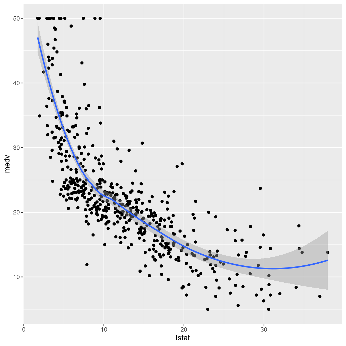
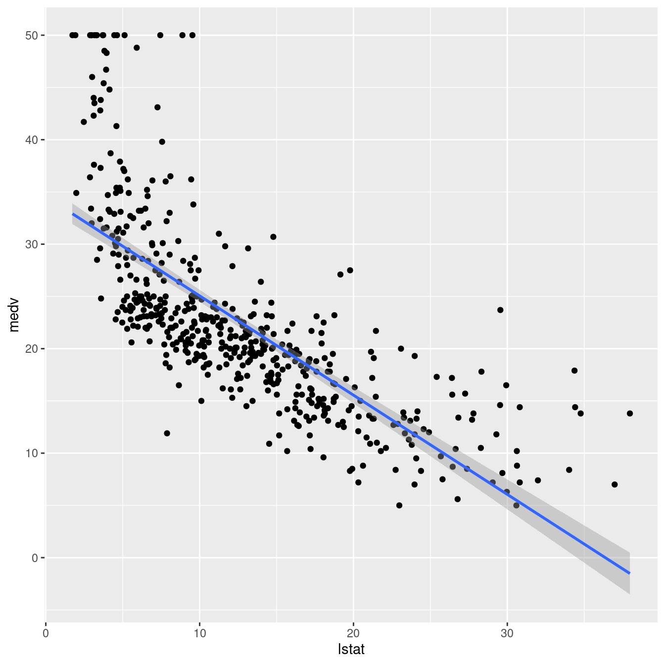
## F-statistic: 108.5 on 10 and 495 DF,  p-value: < 0.00000000000000022

ggplot(boston, aes(lstat, medv) ) +
  geom_point() +
  stat_smooth(method = lm, formula = y ~ poly(x, 5, raw = TRUE))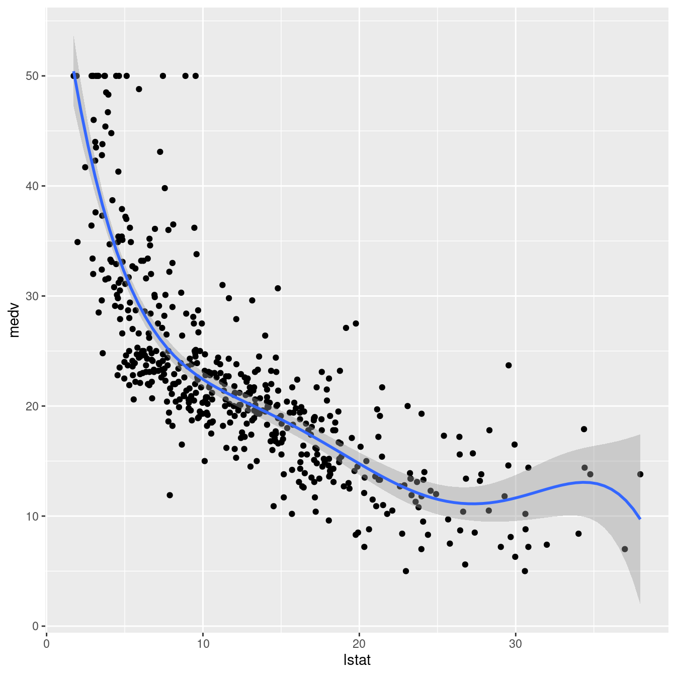

ggplot(boston, aes(lstat, medv) ) +
  geom_point() +
  stat_smooth(method = lm, formula = y ~ log(x))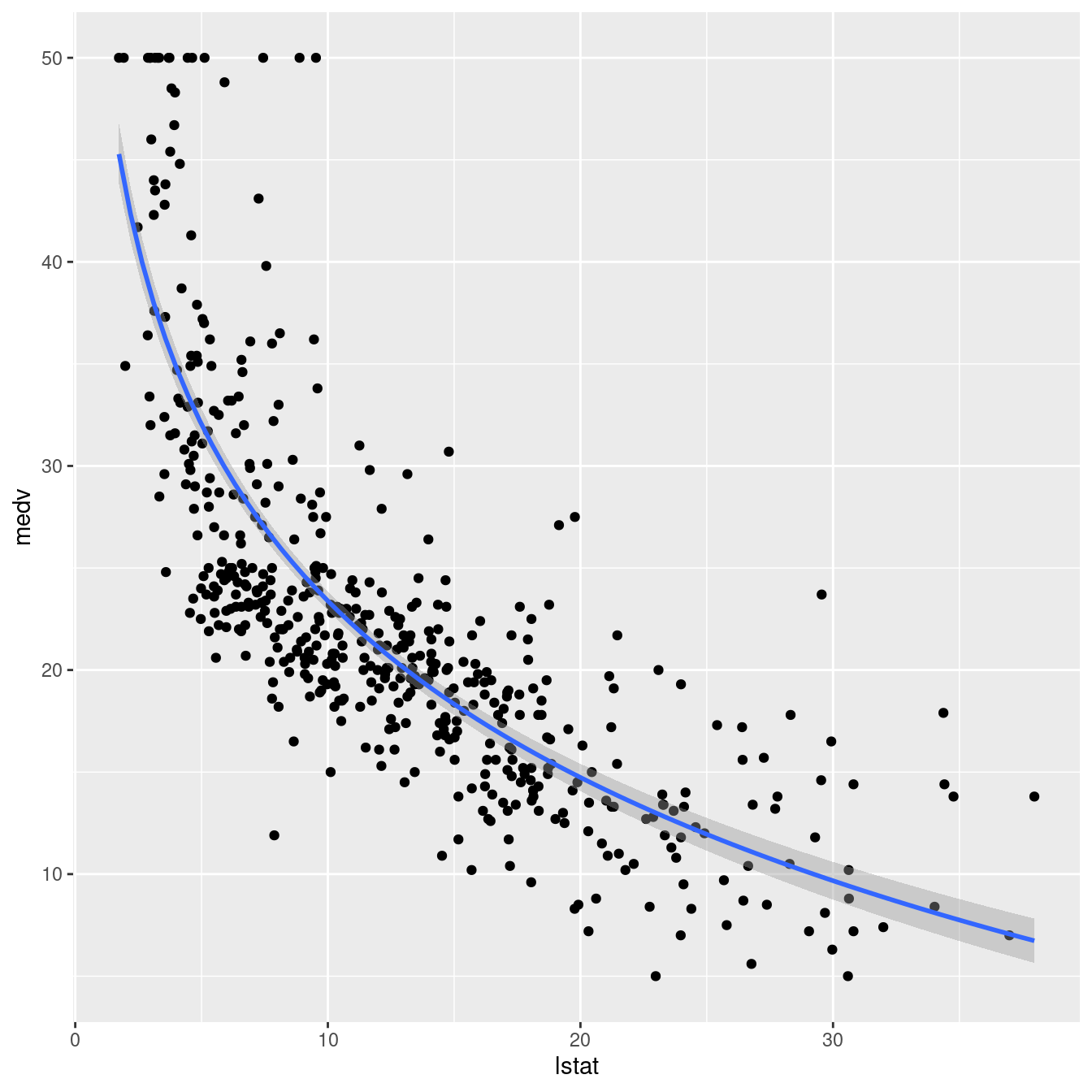

lm(medv ~ log(lstat), data = boston) %>%
  summary()

## 
## Call:
## lm(formula = medv ~ log(lstat), data = boston)
## 
## Residuals:
##      Min       1Q   Median       3Q      Max 
## -14.4599  -3.5006  -0.6686   2.1688  26.0129 
## 
## Coefficients:
##             Estimate Std. Error t value            Pr(>|t|)    
## (Intercept)  52.1248     0.9652   54.00 <0.0000000000000002 ***
## log(lstat)  -12.4810     0.3946  -31.63 <0.0000000000000002 ***
## ---
## Signif. codes:  0 '***' 0.001 '**' 0.01 '*' 0.05 '.' 0.1 ' ' 1
## 
## Residual standard error: 5.329 on 504 degrees of freedom
## Multiple R-squared:  0.6649, Adjusted R-squared:  0.6643 
## F-statistic:  1000 on 1 and 504 DF,  p-value: < 0.00000000000000022

require(mgcv)
ggplot(boston, aes(lstat, medv) ) +
  geom_point() +
  stat_smooth(method = gam, formula = y ~ s(x))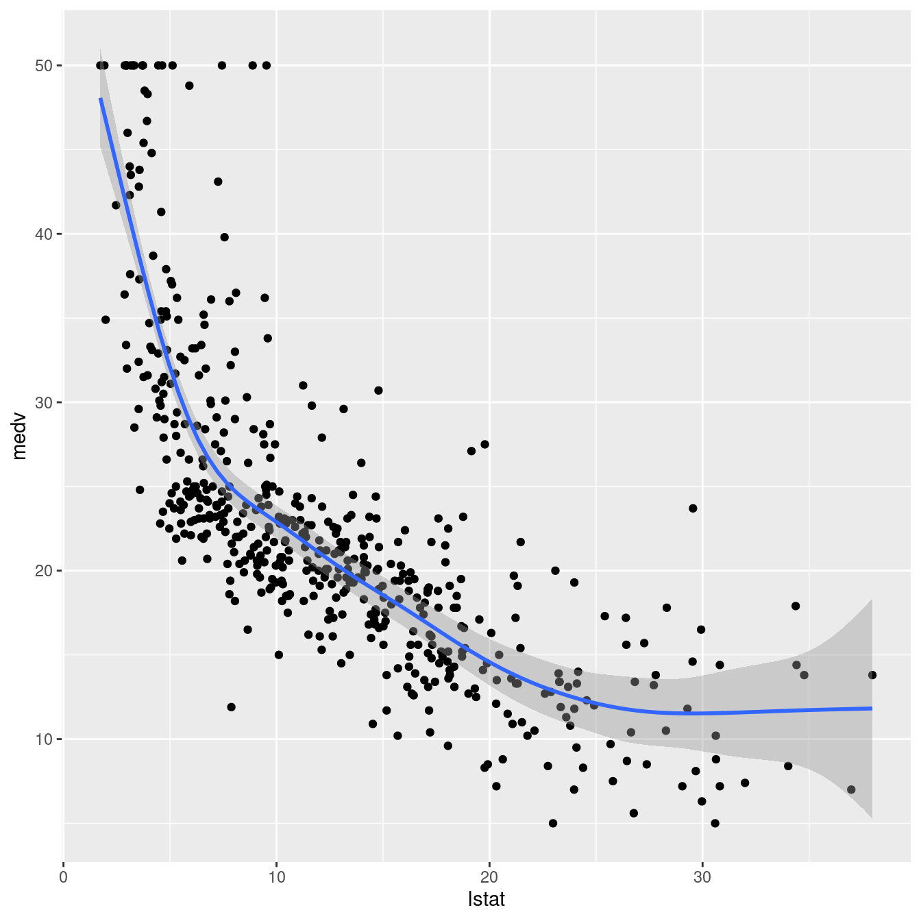

gam(medv ~ s(lstat), data = boston) %>%
  summary()

## 
## Family: gaussian 
## Link function: identity 
## 
## Formula:
## medv ~ s(lstat)
## 
## Parametric coefficients:
##             Estimate Std. Error t value            Pr(>|t|)    
## (Intercept)  22.5328     0.2312   97.47 <0.0000000000000002 ***
## ---
## Signif. codes:  0 '***' 0.001 '**' 0.01 '*' 0.05 '.' 0.1 ' ' 1
## 
## Approximate significance of smooth terms:
##            edf Ref.df     F             p-value    
## s(lstat) 7.403  8.375 128.4 <0.0000000000000002 ***
## ---
## Signif. codes:  0 '***' 0.001 '**' 0.01 '*' 0.05 '.' 0.1 ' ' 1
## 
## R-sq.(adj) =   0.68   Deviance explained = 68.5%
## GCV =   27.5  Scale est. = 27.044    n = 506

14.10 課後練習題