Chapter 15 當簡單線性迴歸遇上機器學習
15.1 旭,劍指「人工智慧」
作者小編在大學時代,「演算法」雖然已經是「計算機概論」這一門課的主角,但是「自己會學習的演算法」、「機器學習」、「深度學習」,甚至是「人工智慧」,聽都沒聽過!好消息是,
演算法進步了!
讓我們先參考Wikipedia怎麼說?
Machine learning (ML) is the study of computer algorithms that improve automatically through experience.
It is seen as a part of artificial intelligence.
Machine learning algorithms build a model based on sample data, known as “training data”, in order to make predictions or decisions without being explicitly programmed to do so.
Machine learning algorithms are used in a wide variety of applications, such as email filtering and computer vision, where it is difficult or unfeasible to develop conventional algorithms to perform the needed tasks.
作者小編的土耳其同學並不認同機器學習!當作者小編知道這事實時,腦門冒出許許多多問號?
為什麼???
15.2 續,劍指「統計學習」
再看看R官方怎麼說?
Several add-on packages implement ideas and methods developed at the borderline between computer science and statistics - this field of research is usually referred to as machine learning.
看到這裡,作者小編最想問的問題是:
What is “borderline between computer science and statistics”?
在這裏有一些答案,說不定有幫助?作者小編先找大分類來刺激大家的「腦門」,也刺激一下作者小編繼續寫作的動機:
- Neural Networks and Deep Learning
- Recursive Partitioning
- Random Forests
- Regularized and Shrinkage Methods
- Boosting and Gradient Descent
- Support Vector Machines and Kernel Methods
- Bayesian Methods
- Optimization using Genetic Algorithms
- Association Rules
- Fuzzy Rule-based Systems
- Model selection and validation
…
15.3 續,劍指「當簡單線性迴歸遇上機器學習」
看過前面兩小段,請讀者諸君特別注意,在Wikipedia,「machine learning」這兩個字劍指
累積經驗自動改善的演算法。
但是,在R,「machine learning」這兩個字劍指
無法手算的統計學。
讀者諸君有「無法手算」的經驗嗎?在這一章,作者小編先示範兩種「無法手算」的統計學:
- Model selection and validation
- Regularized and Shrinkage Methods
關於「Model selection and validation」,作者小編在看過CRAN Task View: Machine Learning & Statistical Learning之後,決定先介紹splitTools: Tools for Data Splitting,因為
切割現有數據集已經被證實是驗證模型最有效的研究方法。
關於「Regularized and Shrinkage Methods」,作者小編嘗試在「簡單線性迴歸線」的框架下,討論
- Ridge
- LASSO
這兩種最經典的方法,並且把焦點放在介紹「超參數」這一個觀念。
什麼是「超參數」呢?
應該先問,
什麼是「參數」呢?
我們在第五章已經知道最小平方法(LS)的
「適當的」
是這個意思
\[\min_{\beta_0, \beta_1} \sum (y - \hat y)^2 = \sum (y - (\beta_0 + \beta_1 \times x))^2\]
接下來,我們,雖然不是作者小編「想要的、想到的、經驗的」,我們想要把前述的
「適當的」
換成
\[\min_{\beta_0, \beta_1} \sum (y - \hat y)^2 = \sum (y - (\beta_0 + \beta_1 \times x))^2, \text{而且}\beta_0 \text{跟}\beta_1 \text{必須滿足} (\beta_0^2 + \beta_1^2) \le c\]
或是改成
\[\min_{\beta_0, \beta_1} \sum (y - \hat y)^2 = \sum (y - (\beta_0 + \beta_1 \times x))^2, \text{而且}\beta_0 \text{跟}\beta_1 \text{必須滿足} (|\beta_0| + |\beta_1|) \le t\]
其中,「\(\beta_0\)」跟「\(\beta_1\)」是所謂的「參數」,而「引進」限制式的參數,可能我們會用「\(\lambda\)」就是所謂的「超參數」。
In machine learning, a hyperparameter (超參數) is a parameter whose value is set before the learning process begins. By contrast, the values of other parameters are derived via training.
另外,作者小編將好好討論「prediction」這一個字。在前面兩章,我們知道「適當的答案」可能是根據
- LS
- Ridge
- LASSO
等三種「標準」找到的!「那時候」,「簡單線性迴歸模型」的用意是
解釋模型,解釋用!
「現在」,假如「簡單線性迴歸模型」的用意「換成」是
預測模型,預測用!
「那」
- LS
- Ridge
- LASSO
依舊可以幫我們找到答案嗎?如果不行,怎麼改?繼續之前,我們先引用這一句話,做做實驗,吸收經驗吧!
Machine learning algorithms build a model based on sample data, known as “training data”, in order to make predictions or decisions without being explicitly programmed to do so.
…
15.5 準備工作
- 波士頓數據集。
require(MASS) # 用「require」不用「library」,是因為如果R已經將套件MASS載入環境,就不需要再載一次。
data(Boston)
boston <- Boston
# 「不動」原始數據集,不論它有「多原始」,是R程式設計的一項絕佳習慣。
# 即便一般使用者是無法任意改變套件MASS的內容物!
### rad (index of accessibility to radial highways)
boston[,"rad"] <- factor(boston[,"rad"], ordered = TRUE)
### chas (= 1 if tract bounds river; 0 otherwise)
boston[,"chas"] <- factor(boston[,"chas"])
head(boston)
## crim zn indus chas nox rm age dis rad tax ptratio black lstat
## 1 0.00632 18 2.31 0 0.538 6.575 65.2 4.0900 1 296 15.3 396.90 4.98
## 2 0.02731 0 7.07 0 0.469 6.421 78.9 4.9671 2 242 17.8 396.90 9.14
## 3 0.02729 0 7.07 0 0.469 7.185 61.1 4.9671 2 242 17.8 392.83 4.03
## 4 0.03237 0 2.18 0 0.458 6.998 45.8 6.0622 3 222 18.7 394.63 2.94
## 5 0.06905 0 2.18 0 0.458 7.147 54.2 6.0622 3 222 18.7 396.90 5.33
## 6 0.02985 0 2.18 0 0.458 6.430 58.7 6.0622 3 222 18.7 394.12 5.21
## medv
## 1 24.0
## 2 21.6
## 3 34.7
## 4 33.4
## 5 36.2
## 6 28.7tail(boston)## crim zn indus chas nox rm age dis rad tax ptratio black lstat
## 501 0.22438 0 9.69 0 0.585 6.027 79.7 2.4982 6 391 19.2 396.90 14.33
## 502 0.06263 0 11.93 0 0.573 6.593 69.1 2.4786 1 273 21.0 391.99 9.67
## 503 0.04527 0 11.93 0 0.573 6.120 76.7 2.2875 1 273 21.0 396.90 9.08
## 504 0.06076 0 11.93 0 0.573 6.976 91.0 2.1675 1 273 21.0 396.90 5.64
## 505 0.10959 0 11.93 0 0.573 6.794 89.3 2.3889 1 273 21.0 393.45 6.48
## 506 0.04741 0 11.93 0 0.573 6.030 80.8 2.5050 1 273 21.0 396.90 7.88
## medv
## 501 16.8
## 502 22.4
## 503 20.6
## 504 23.9
## 505 22.0
## 506 11.9### 讀取自製的波士頓數據集中文資訊。
DISvars <- colnames(boston)[which(sapply(boston, class) == "integer")]
CONvars <- colnames(boston)[which(sapply(boston, class) == "numeric")]
colsBostonFull<-readRDS("output/data/colsBostonFull.rds")
colsBostonFull$內容物 <- sapply(boston, class)
colsBostonFull## 變數名
## 1 crim
## 2 zn
## 3 indus
## 4 chas
## 5 nox
## 6 rm
## 7 age
## 8 dis
## 9 rad
## 10 tax
## 11 ptratio
## 12 black
## 13 lstat
## 14 medv
## 說明
## 1 per capita crime rate by town
## 2 proportion of residential land zoned for lots over 25,000 sq.ft.
## 3 proportion of non-retail business acres per town
## 4 Charles River dummy variable (= 1 if tract bounds river; 0 otherwise)
## 5 nitric oxides concentration (parts per 10 million)
## 6 average number of rooms per dwelling
## 7 proportion of owner-occupied units built prior to 1940
## 8 weighted distances to five Boston employment centres
## 9 index of accessibility to radial highways
## 10 full-value property-tax rate per $10,000
## 11 pupil-teacher ratio by town
## 12 1000(Bk - 0.63)^2 where Bk is the proportion of blacks by town
## 13 % lower status of the population
## 14 Median value of owner-occupied homes in $1000's
## 中文翻譯 中文變數名稱 內容物
## 1 每個城鎮人均犯罪率。 犯罪率 numeric
## 2 超過25,000平方呎的住宅用地比例。 住宅用地比例 numeric
## 3 每個城鎮非零售業務英畝的比例。 非商業區比例 numeric
## 4 是否鄰近Charles River。 河邊宅 factor
## 5 氮氧化合物濃度。 空汙指標 numeric
## 6 每個住宅的平均房間數。 平均房間數 numeric
## 7 1940年之前建造的自用住宅比例。 老房子比例 numeric
## 8 距波士頓五大商圈的加權平均距離。 加權平均距離 numeric
## 9 環狀高速公路的可觸指標。 交通便利性 ordered, factor
## 10 財產稅占比(每一萬美元)。 財產稅率 numeric
## 11 生師比。 生師比 numeric
## 12 黑人的比例。 黑人指數 numeric
## 13 (比較)低社經地位人口的比例。 低社經人口比例 numeric
## 14 以千美元計的房價中位數。 房價中位數 numeric- Anscombe數據集。
require(datasets) # 通常我們是這麼寫「library(datasets)」。
data("anscombe") # 載入。
anscombe # 呼叫它。
## x1 x2 x3 x4 y1 y2 y3 y4
## 1 10 10 10 8 8.04 9.14 7.46 6.58
## 2 8 8 8 8 6.95 8.14 6.77 5.76
## 3 13 13 13 8 7.58 8.74 12.74 7.71
## 4 9 9 9 8 8.81 8.77 7.11 8.84
## 5 11 11 11 8 8.33 9.26 7.81 8.47
## 6 14 14 14 8 9.96 8.10 8.84 7.04
## 7 6 6 6 8 7.24 6.13 6.08 5.25
## 8 4 4 4 19 4.26 3.10 5.39 12.50
## 9 12 12 12 8 10.84 9.13 8.15 5.56
## 10 7 7 7 8 4.82 7.26 6.42 7.91
## 11 5 5 5 8 5.68 4.74 5.73 6.89df <- anscombe[, c("x1", "y1")] # 取出「x1」跟「y1」,其中「1」代表第一組。
colnames(df) <- c("x", "y") # 劃掉其中的「1」。
df # 呼叫出來再一次檢視這一組數據集。## x y
## 1 10 8.04
## 2 8 6.95
## 3 13 7.58
## 4 9 8.81
## 5 11 8.33
## 6 14 9.96
## 7 6 7.24
## 8 4 4.26
## 9 12 10.84
## 10 7 4.82
## 11 5 5.68m0 <- lm(y ~ x, data = df)
summary(m0)##
## Call:
## lm(formula = y ~ x, data = df)
##
## Residuals:
## Min 1Q Median 3Q Max
## -1.92127 -0.45577 -0.04136 0.70941 1.83882
##
## Coefficients:
## Estimate Std. Error t value Pr(>|t|)
## (Intercept) 3.0001 1.1247 2.667 0.02573 *
## x 0.5001 0.1179 4.241 0.00217 **
## ---
## Signif. codes: 0 '***' 0.001 '**' 0.01 '*' 0.05 '.' 0.1 ' ' 1
##
## Residual standard error: 1.237 on 9 degrees of freedom
## Multiple R-squared: 0.6665, Adjusted R-squared: 0.6295
## F-statistic: 17.99 on 1 and 9 DF, p-value: 0.00217…
15.6 請套件splitTools協助切割數據集
- data partitioning (e.g. into training, validation and test),
- creating folds for cross-validation,
- creating repeated folds for cross-validation,
- stratified splitting (e.g. for stratified cross-validation),
- grouped splitting (e.g. for group-k-fold cross-validation),
- blocked splitting (if the sequential order of the data should be retained),
- time-series splitting where the out-of-sample data follows the (growing) in-sample data.
15.6.1 切:data partitioning (e.g. into training and test)
require(splitTools)
# Split into training and test
set.seed(3451)
inds <- partition(df$y, p = c(train = 0.8, test = 0.2))
str(inds)## List of 2
## $ train: int [1:7] 2 3 4 5 7 9 11
## $ test : int [1:4] 1 6 8 10train <- df[inds$train, ]
train[order(train$y), ]## x y
## 11 5 5.68
## 2 8 6.95
## 7 6 7.24
## 3 13 7.58
## 5 11 8.33
## 4 9 8.81
## 9 12 10.84test <- df[inds$test, ]
test[order(test$y), ]## x y
## 8 4 4.26
## 10 7 4.82
## 1 10 8.04
## 6 14 9.9615.6.2 切:data partitioning (e.g. into training, validation and test)
require(splitTools)
# Split data into partitions
set.seed(3451)
inds <- partition(df$y, p = c(train = 0.6, valid = 0.2, test = 0.2))
str(inds)## List of 3
## $ train: int [1:5] 2 3 4 7 9
## $ valid: int 8
## $ test : int [1:5] 1 5 6 10 11train <- df[inds$train, ]
train[order(train$y), ]## x y
## 2 8 6.95
## 7 6 7.24
## 3 13 7.58
## 4 9 8.81
## 9 12 10.84valid <- df[inds$valid, ]
valid[order(valid$y), ]## x y
## 8 4 4.26test <- df[inds$test, ]
test[order(test$y), ]## x y
## 10 7 4.82
## 11 5 5.68
## 1 10 8.04
## 5 11 8.33
## 6 14 9.9615.6.3 切:stratified splitting (e.g. for stratified cross-validation)
require(splitTools)
# Split into training and test
set.seed(3451)
inds <- partition(df$y, p = c(train = 0.8, test = 0.2))
str(inds)## List of 2
## $ train: int [1:7] 2 3 4 5 7 9 11
## $ test : int [1:4] 1 6 8 10train <- df[inds$train, ]
train[order(train$y), ]## x y
## 11 5 5.68
## 2 8 6.95
## 7 6 7.24
## 3 13 7.58
## 5 11 8.33
## 4 9 8.81
## 9 12 10.84test <- df[inds$test, ]
test[order(test$y), ]## x y
## 8 4 4.26
## 10 7 4.82
## 1 10 8.04
## 6 14 9.96# Get stratified cross-validation fold indices
folds <- create_folds(train$y, k = 2)
folds## $Fold1
## [1] 1 2 5 6
##
## $Fold2
## [1] 3 4 7train## x y
## 2 8 6.95
## 3 13 7.58
## 4 9 8.81
## 5 11 8.33
## 7 6 7.24
## 9 12 10.84
## 11 5 5.68train[folds[[1]], ]## x y
## 2 8 6.95
## 3 13 7.58
## 7 6 7.24
## 9 12 10.84train[folds[[2]], ]## x y
## 4 9 8.81
## 5 11 8.33
## 11 5 5.6815.6.4 切:creating repeated folds for cross-validation
require(splitTools)
# Split into training and test
set.seed(3451)
inds <- partition(df$y, p = c(train = 0.8, test = 0.2))
str(inds)## List of 2
## $ train: int [1:7] 2 3 4 5 7 9 11
## $ test : int [1:4] 1 6 8 10train <- df[inds$train, ]
train[order(train$y), ]## x y
## 11 5 5.68
## 2 8 6.95
## 7 6 7.24
## 3 13 7.58
## 5 11 8.33
## 4 9 8.81
## 9 12 10.84test <- df[inds$test, ]
test[order(test$y), ]## x y
## 8 4 4.26
## 10 7 4.82
## 1 10 8.04
## 6 14 9.96# Get srepeated, stratified cross-validation folds of indices
folds <- create_folds(train$y, k = 2, m_rep = 5)
folds## $Fold1.Rep1
## [1] 1 2 5 6
##
## $Fold2.Rep1
## [1] 3 4 7
##
## $Fold1.Rep2
## [1] 1 2 6 7
##
## $Fold2.Rep2
## [1] 3 4 5
##
## $Fold1.Rep3
## [1] 6 7
##
## $Fold2.Rep3
## [1] 1 2 3 4 5
##
## $Fold1.Rep4
## [1] 7
##
## $Fold2.Rep4
## [1] 1 2 3 4 5 6
##
## $Fold1.Rep5
## [1] 2 4 5 7
##
## $Fold2.Rep5
## [1] 1 3 6train## x y
## 2 8 6.95
## 3 13 7.58
## 4 9 8.81
## 5 11 8.33
## 7 6 7.24
## 9 12 10.84
## 11 5 5.68train[folds[[1]], ]## x y
## 2 8 6.95
## 3 13 7.58
## 7 6 7.24
## 9 12 10.84train[folds[[2]], ]## x y
## 4 9 8.81
## 5 11 8.33
## 11 5 5.6815.6.5 切:time-series cross-validation and block partitioning
require(splitTools)
# Block partitioning
set.seed(3451)
inds <- partition(df$y,
p = c(train = 0.8, test = 0.2),
type = "blocked")
str(inds)## List of 2
## $ train: int [1:9] 1 2 3 4 5 6 7 8 9
## $ test : int [1:2] 10 11train <- df[inds$train, ]
train[order(train$y), ]## x y
## 8 4 4.26
## 2 8 6.95
## 7 6 7.24
## 3 13 7.58
## 1 10 8.04
## 5 11 8.33
## 4 9 8.81
## 6 14 9.96
## 9 12 10.84test <- df[inds$test, ]
test[order(test$y), ]## x y
## 10 7 4.82
## 11 5 5.68# Get time series folds
folds <- create_timefolds(train$y, k = 2)
str(folds)## List of 2
## $ Fold1:List of 2
## ..$ insample : int [1:3] 1 2 3
## ..$ outsample: int [1:3] 4 5 6
## $ Fold2:List of 2
## ..$ insample : int [1:6] 1 2 3 4 5 6
## ..$ outsample: int [1:3] 7 8 9folds## $Fold1
## $Fold1$insample
## [1] 1 2 3
##
## $Fold1$outsample
## [1] 4 5 6
##
##
## $Fold2
## $Fold2$insample
## [1] 1 2 3 4 5 6
##
## $Fold2$outsample
## [1] 7 8 9train## x y
## 1 10 8.04
## 2 8 6.95
## 3 13 7.58
## 4 9 8.81
## 5 11 8.33
## 6 14 9.96
## 7 6 7.24
## 8 4 4.26
## 9 12 10.84train[folds[[1]][[1]], ]## x y
## 1 10 8.04
## 2 8 6.95
## 3 13 7.58train[folds[[1]][[2]], ]## x y
## 4 9 8.81
## 5 11 8.33
## 6 14 9.9615.7 示範「Regularized and Shrinkage Methods」
15.7.1 準備「Regularized and Shrinkage Methods」的示範數據
df <- anscombe[, c("x1", "y1")] # 取出「x1」跟「y1」,其中「1」代表第一組。
colnames(df) <- c("x", "y") # 劃掉其中的「1」。
df # 呼叫出來再一次檢視這一組數據集。
## x y
## 1 10 8.04
## 2 8 6.95
## 3 13 7.58
## 4 9 8.81
## 5 11 8.33
## 6 14 9.96
## 7 6 7.24
## 8 4 4.26
## 9 12 10.84
## 10 7 4.82
## 11 5 5.68# 繪製散佈圖。左右上下各加3個單位,方便大家觀察。
plot(df,
xlim = range(df[, "x"]) + c(-3, 3),
ylim = range(df[, "y"]) + c(-3, 3),
type = "n")
text(df,
labels = 1:dim(df)[1],
cex = 0.8)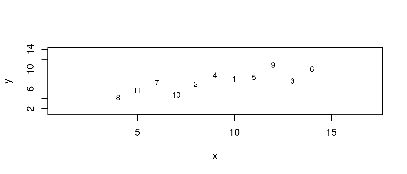
df[1:2, c("x", "y")] # 先看座標。## x y
## 1 10 8.04
## 2 8 6.95b <- diff(df[1:2,"y"])/diff(df[1:2,"x"]) # 直接翻譯上述答案。「斜率」等於「y座標的差距」除以「x座標的差距」。
a <- df[1,"y"] - b * df[1,"x"] # 「截距」等於第一點的y座標減去斜率乘以第一點的x座標。
LINE <- c(a, b) # 報告成果。
names(LINE) <- c("a", "b")
LINE## a b
## 2.590 0.545for (i in 1:11) {
for (j in 1:11) {
if(i == j) {
next
} else {
b <- diff(df[c(i,j),"y"])/diff(df[c(i,j),"x"])
# 直接翻譯上述答案。
#「斜率」等於「y座標的差距」除以「x座標的差距」。
a <- df[i,"y"] - b * df[i,"x"]
#「截距」等於第一點的y座標減去斜率乘以第一點的x座標。
LINE <- c(a, b) # 報告成果。
names(LINE) <- c("a", "b")
print(LINE)
}
}
}## a b
## 2.590 0.545
## a b
## 9.5733333 -0.1533333
## a b
## 15.74 -0.77
## a b
## 5.14 0.29
## a b
## 3.24 0.48
## a b
## 6.04 0.20
## a b
## 1.74 0.63
## a b
## -5.96 1.40
## a b
## -2.693333 1.073333
## a b
## 3.320 0.472
##     a     b
## 2.590 0.545
## a b
## 5.942 0.126
## a b
## -7.93 1.86
## a b
## 3.27 0.46
## a b
## 2.9366667 0.5016667
## a b
## 8.110 -0.145
## a b
## 1.5700 0.6725
## a b
## -0.8300 0.9725
## a b
## -10.09 2.13
## a b
## 3.5633333 0.4233333
## a b
## 9.5733333 -0.1533333
## a b
## 5.942 0.126
## a b
## 11.5775 -0.3075
## a b
## 12.455 -0.375
## a b
## -23.36 2.38
## a b
## 6.94857143 0.04857143
## a b
## 2.7844444 0.3688889
## a b
## 49.96 -3.26
## a b
## 1.60 0.46
## a b
## 4.4925 0.2375
## a b
## 15.74 -0.77
## a b
## -7.93 1.86
## a b
## 11.5775 -0.3075
## a b
## 10.97 -0.24
## a b
## 6.74 0.23
## a b
## 4.1000000 0.5233333
## a b
## 0.62 0.91
## a b
## 2.7200000 0.6766667
## a b
## -9.145 1.995
## a b
## 1.7675 0.7825
## a b
## 5.14 0.29
## a b
## 3.27 0.46
## a b
## 12.455 -0.375
## a b
## 10.97 -0.24
## a b
## 2.3533333 0.5433333
## a b
## 5.932 0.218
## a b
## 1.9342857 0.5814286
## a b
## -19.28 2.51
## a b
## -1.3225 0.8775
## a b
## 3.4716667 0.4416667
## a b
## 3.24 0.48
## a b
## 2.9366667 0.5016667
## a b
## -23.36 2.38
## a b
## 6.74 0.23
## a b
## 2.3533333 0.5433333
## a b
## 5.20 0.34
## a b
## 1.98 0.57
## a b
## 16.12 -0.44
## a b
## -0.3200000 0.7342857
## a b
## 3.3022222 0.4755556
## a b
## 6.04 0.20
## a b
## 8.110 -0.145
## a b
## 6.94857143 0.04857143
## a b
## 4.1000000 0.5233333
## a b
## 5.932 0.218
## a b
## 5.20 0.34
## a b
## -1.70 1.49
## a b
## 3.64 0.60
## a b
## 21.76 -2.42
## a b
## -2.12 1.56
## a b
## 1.74 0.63
## a b
## 1.5700 0.6725
## a b
## 2.7844444 0.3688889
## a b
## 0.62 0.91
## a b
## 1.9342857 0.5814286
## a b
## 1.98 0.57
## a b
## -1.70 1.49
## a b
## 0.9700 0.8225
## a b
## 3.5133333 0.1866667
## a b
## -1.42 1.42
## a b
## -5.96 1.40
## a b
## -0.8300 0.9725
## a b
## 49.96 -3.26
## a b
## 2.7200000 0.6766667
## a b
## -19.28 2.51
## a b
## 16.12 -0.44
## a b
## 3.64 0.60
## a b
## 0.9700 0.8225
## a b
## -3.608 1.204
## a b
## 1.9942857 0.7371429
## a b
## -2.693333 1.073333
## a b
## -10.09 2.13
## a b
## 1.60 0.46
## a b
## -9.145 1.995
## a b
## -1.3225 0.8775
## a b
## -0.3200000 0.7342857
## a b
## 21.76 -2.42
## a b
## 3.5133333 0.1866667
## a b
## -3.608 1.204
## a b
## 7.83 -0.43
## a b
## 3.320 0.472
## a b
## 3.5633333 0.4233333
## a b
## 4.4925 0.2375
## a b
## 1.7675 0.7825
## a b
## 3.4716667 0.4416667
## a b
## 3.3022222 0.4755556
## a b
## -2.12 1.56
## a b
## -1.42 1.42
## a b
## 1.9942857 0.7371429
## a b
## 7.83 -0.4315.7.2 Ridge思維
\[\min_{\beta_0, \beta_1} \sum (y - \hat y)^2 = \sum (y - (\beta_0 + \beta_1 \times x))^2, \text{而且}\beta_0 \text{跟}\beta_1 \text{必須滿足} (\beta_0^2 + \beta_1^2) \le c\]
等同於
\[\min_{\beta_0, \beta_1} \sum (y - (\beta_0 + \beta_1 \times x))^2 + \lambda (\beta_0^2 + \beta_1^2)\]
LINES <- data.frame(a = numeric(0),
                    b = numeric(0),
                    a2 = numeric(0),
                    b2 = numeric(0),
                    ridge = numeric(0),
                    sse = numeric(0))
for (i in 1:11) {
  for (j in 1:11) {
    if(i == j) {
      next
    } else {
      b <- diff(df[c(i,j),"y"])/diff(df[c(i,j),"x"])
      # 直接翻譯上述答案。
      #「斜率」等於「y座標的差距」除以「x座標的差距」。
      a <- df[i,"y"] - b * df[i,"x"]
      #「截距」等於第一點的y座標減去斜率乘以第一點的x座標。
      LINE <- c(a, b) # 報告成果。
      names(LINE) <- c("a", "b")
      SSE <- sum((df$y - (a + b * df$x))^2)
      LINE0 <- data.frame(a = a,
                          b = b,
                          a2 = a^2,
                          b2 = b^2,
                          ridge = a^2+b^2,
                          sse = SSE)
      LINES <- rbind(LINES, LINE0)

    }

  }
}
LINES[order(LINES$sse), ]
## a b a2 b2 ridge sse
## 15 2.936667 0.50166667 8.624011 0.251669444 8.8756806 13.78964
## 52 2.936667 0.50166667 8.624011 0.251669444 8.8756806 13.78964
## 5 3.240000 0.48000000 10.497600 0.230400000 10.7280000 13.84550
## 51 3.240000 0.48000000 10.497600 0.230400000 10.7280000 13.84550
## 10 3.320000 0.47200000 11.022400 0.222784000 11.2451840 13.89900
## 101 3.320000 0.47200000 11.022400 0.222784000 11.2451840 13.89900
## 60 3.302222 0.47555556 10.904672 0.226153086 11.1308247 13.90164
## 106 3.302222 0.47555556 10.904672 0.226153086 11.1308247 13.90164
## 1 2.590000 0.54500000 6.708100 0.297025000 7.0051250 13.98492
## 11 2.590000 0.54500000 6.708100 0.297025000 7.0051250 13.98492
## 14 3.270000 0.46000000 10.692900 0.211600000 10.9045000 14.03040
## 42 3.270000 0.46000000 10.692900 0.211600000 10.9045000 14.03040
## 50 3.471667 0.44166667 12.052469 0.195069444 12.2475389 14.17053
## 105 3.471667 0.44166667 12.052469 0.195069444 12.2475389 14.17053
## 20 3.563333 0.42333333 12.697344 0.179211111 12.8765556 14.58981
## 102 3.563333 0.42333333 12.697344 0.179211111 12.8765556 14.58981
## 45 2.353333 0.54333333 5.538178 0.295211111 5.8333889 14.69818
## 55 2.353333 0.54333333 5.538178 0.295211111 5.8333889 14.69818
## 7 1.740000 0.63000000 3.027600 0.396900000 3.4245000 15.71000
## 71 1.740000 0.63000000 3.027600 0.396900000 3.4245000 15.71000
## 75 1.934286 0.58142857 3.741461 0.338059184 4.0795204 15.71583
## 47 1.934286 0.58142857 3.741461 0.338059184 4.0795204 15.71583
## 57 1.980000 0.57000000 3.920400 0.324900000 4.2453000 15.98120
## 76 1.980000 0.57000000 3.920400 0.324900000 4.2453000 15.98120
## 17 1.570000 0.67250000 2.464900 0.452256250 2.9171562 17.19506
## 72 1.570000 0.67250000 2.464900 0.452256250 2.9171562 17.19506
## 4 5.140000 0.29000000 26.419600 0.084100000 26.5037000 19.30040
## 41 5.140000 0.29000000 26.419600 0.084100000 26.5037000 19.30040
## 56 5.200000 0.34000000 27.040000 0.115600000 27.1556000 22.92030
## 66 5.200000 0.34000000 27.040000 0.115600000 27.1556000 22.92030
## 46 5.932000 0.21800000 35.188624 0.047524000 35.2361480 24.21570
## 65 5.932000 0.21800000 35.188624 0.047524000 35.2361480 24.21570
## 6 6.040000 0.20000000 36.481600 0.040000000 36.5216000 24.93350
## 61 6.040000 0.20000000 36.481600 0.040000000 36.5216000 24.93350
## 30 4.492500 0.23750000 20.182556 0.056406250 20.2389625 29.69094
## 103 4.492500 0.23750000 20.182556 0.056406250 20.2389625 29.69094
## 12 5.942000 0.12600000 35.307364 0.015876000 35.3232400 31.14256
## 22 5.942000 0.12600000 35.307364 0.015876000 35.3232400 31.14256
## 36 4.100000 0.52333333 16.810000 0.273877778 17.0838778 32.67302
## 64 4.100000 0.52333333 16.810000 0.273877778 17.0838778 32.67302
## 88 0.970000 0.82250000 0.940900 0.676506250 1.6174062 33.55331
## 78 0.970000 0.82250000 0.940900 0.676506250 1.6174062 33.55331
## 90 1.994286 0.73714286 3.977176 0.543379592 4.5205551 33.93183
## 109 1.994286 0.73714286 3.977176 0.543379592 4.5205551 33.93183
## 59 -0.320000 0.73428571 0.102400 0.539175510 0.6415755 35.96327
## 96 -0.320000 0.73428571 0.102400 0.539175510 0.6415755 35.96327
## 38 2.720000 0.67666667 7.398400 0.457877778 7.8562778 36.04329
## 84 2.720000 0.67666667 7.398400 0.457877778 7.8562778 36.04329
## 26 6.948571 0.04857143 48.282645 0.002359184 48.2850041 36.33434
## 63 6.948571 0.04857143 48.282645 0.002359184 48.2850041 36.33434
## 73 2.784444 0.36888889 7.753131 0.136079012 7.8892099 37.10748
## 27 2.784444 0.36888889 7.753131 0.136079012 7.8892099 37.10748
## 49 -1.322500 0.87750000 1.749006 0.770006250 2.5190125 38.86121
## 95 -1.322500 0.87750000 1.749006 0.770006250 2.5190125 38.86121
## 18 -0.830000 0.97250000 0.688900 0.945756250 1.6346562 40.26656
## 82 -0.830000 0.97250000 0.688900 0.945756250 1.6346562 40.26656
## 35 6.740000 0.23000000 45.427600 0.052900000 45.4805000 40.63800
## 54 6.740000 0.23000000 45.427600 0.052900000 45.4805000 40.63800
## 68 3.640000 0.60000000 13.249600 0.360000000 13.6096000 40.91750
## 87 3.640000 0.60000000 13.249600 0.360000000 13.6096000 40.91750
## 40 1.767500 0.78250000 3.124056 0.612306250 3.7363625 41.38664
## 104 1.767500 0.78250000 3.124056 0.612306250 3.7363625 41.38664
## 29 1.600000 0.46000000 2.560000 0.211600000 2.7716000 48.04830
## 93 1.600000 0.46000000 2.560000 0.211600000 2.7716000 48.04830
## 37 0.620000 0.91000000 0.384400 0.828100000 1.2125000 51.09640
## 74 0.620000 0.91000000 0.384400 0.828100000 1.2125000 51.09640
## 91 -2.693333 1.07333333 7.254044 1.152044444 8.4060889 53.04901
## 9 -2.693333 1.07333333 7.254044 1.152044444 8.4060889 53.04901
## 16 8.110000 -0.14500000 65.772100 0.021025000 65.7931250 64.86553
## 62 8.110000 -0.14500000 65.772100 0.021025000 65.7931250 64.86553
## 2 9.573333 -0.15333333 91.648711 0.023511111 91.6722222 66.00261
## 21 9.573333 -0.15333333 91.648711 0.023511111 91.6722222 66.00261
## 89 -3.608000 1.20400000 13.017664 1.449616000 14.4672800 69.08564
## 99 -3.608000 1.20400000 13.017664 1.449616000 14.4672800 69.08564
## 79 3.513333 0.18666667 12.343511 0.034844444 12.3783556 83.14248
## 98 3.513333 0.18666667 12.343511 0.034844444 12.3783556 83.14248
## 34 10.970000 -0.24000000 120.340900 0.057600000 120.3985000 92.86440
## 44 10.970000 -0.24000000 120.340900 0.057600000 120.3985000 92.86440
## 23 11.577500 -0.30750000 134.038506 0.094556250 134.1330625 104.35594
## 33 11.577500 -0.30750000 134.038506 0.094556250 134.1330625 104.35594
## 8 -5.960000 1.40000000 35.521600 1.960000000 37.4816000 110.99750
## 81 -5.960000 1.40000000 35.521600 1.960000000 37.4816000 110.99750
## 24 12.455000 -0.37500000 155.127025 0.140625000 155.2676500 125.42775
## 43 12.455000 -0.37500000 155.127025 0.140625000 155.2676500 125.42775
## 3 15.740000 -0.77000000 247.747600 0.592900000 248.3405000 210.05800
## 31 15.740000 -0.77000000 247.747600 0.592900000 248.3405000 210.05800
## 13 -7.930000 1.86000000 62.884900 3.459600000 66.3445000 236.04240
## 32 -7.930000 1.86000000 62.884900 3.459600000 66.3445000 236.04240
## 100 7.830000 -0.43000000 61.308900 0.184900000 61.4938000 246.83870
## 110 7.830000 -0.43000000 61.308900 0.184900000 61.4938000 246.83870
## 80 -1.420000 1.42000000 2.016400 2.016400000 4.0328000 270.66670
## 108 -1.420000 1.42000000 2.016400 2.016400000 4.0328000 270.66670
## 39 -9.145000 1.99500000 83.631025 3.980025000 87.6110500 278.43645
## 94 -9.145000 1.99500000 83.631025 3.980025000 87.6110500 278.43645
## 67 -1.700000 1.49000000 2.890000 2.220100000 5.1101000 316.43480
## 77 -1.700000 1.49000000 2.890000 2.220100000 5.1101000 316.43480
## 19 -10.090000 2.13000000 101.808100 4.536900000 106.3450000 333.41790
## 92 -10.090000 2.13000000 101.808100 4.536900000 106.3450000 333.41790
## 58 16.120000 -0.44000000 259.854400 0.193600000 260.0480000 349.75590
## 86 16.120000 -0.44000000 259.854400 0.193600000 260.0480000 349.75590
## 70 -2.120000 1.56000000 4.494400 2.433600000 6.9280000 352.14950
## 107 -2.120000 1.56000000 4.494400 2.433600000 6.9280000 352.14950
## 85 -19.280000 2.51000000 371.718400 6.300100000 378.0185000 651.33440
## 48 -19.280000 2.51000000 371.718400 6.300100000 378.0185000 651.33440
## 53 -23.360000 2.38000000 545.689600 5.664400000 551.3540000 1382.94750
## 25 -23.360000 2.38000000 545.689600 5.664400000 551.3540000 1382.94750
## 69 21.760000 -2.42000000 473.497600 5.856400000 479.3540000 1573.92990
## 97 21.760000 -2.42000000 473.497600 5.856400000 479.3540000 1573.92990
## 28 49.960000 -3.26000000 2496.001600 10.627600000 2506.6292000 3462.18990
## 83 49.960000 -3.26000000 2496.001600 10.627600000 2506.6292000 3462.18990LINESls <- data.frame(a = numeric(0),
b = numeric(0),
a2 = numeric(0),
b2 = numeric(0),
ridge = numeric(0),
sse = numeric(0))
df <- rbind(df, c(mean(df$x), mean(df$y)))
df## x y
## 1 10 8.040000
## 2 8 6.950000
## 3 13 7.580000
## 4 9 8.810000
## 5 11 8.330000
## 6 14 9.960000
## 7 6 7.240000
## 8 4 4.260000
## 9 12 10.840000
## 10 7 4.820000
## 11 5 5.680000
## 12 9 7.500909for (i in 1:11) {
b <- diff(df[c(i,12),"y"])/diff(df[c(i,12),"x"])
# 直接翻譯上述答案。
#「斜率」等於「y座標的差距」除以「x座標的差距」。
a <- df[i,"y"] - b * df[i,"x"]
#「截距」等於第一點的y座標減去斜率乘以第一點的x座標。
LINE <- c(a, b) # 報告成果。
names(LINE) <- c("a", "b")
SSE <- sum((df$y - (a + b * df$x))^2)
LINE0 <- data.frame(a = a,
b = b,
a2 = a^2,
b2 = b^2,
ridge = a^2+b^2,
sse = SSE)
LINESls <- rbind(LINESls, LINE0)
}
LINESls[order(LINESls$sse), ]## a b a2 b2 ridge sse
## 6 3.074545 0.49181818 9.452830 0.2418851240 9.694715 13.77022
## 1 2.649091 0.53909091 7.017683 0.2906190083 7.308302 13.93000
## 11 3.403864 0.45522727 11.586288 0.2072318698 11.793520 13.98409
## 2 2.542727 0.55090909 6.465462 0.3035008264 6.768963 14.04676
## 5 3.770000 0.41454545 14.212900 0.1718479339 14.384748 14.56767
## 8 1.667273 0.64818182 2.779798 0.4201396694 3.199938 16.17509
## 7 6.718182 0.08696970 45.133967 0.0075637282 45.141531 32.53629
## 3 7.322955 0.01977273 53.625663 0.0003909607 53.626054 39.14030
## 9 -2.516364 1.11303030 6.332086 1.2388364555 7.570922 55.08911
## 10 -4.563182 1.34045455 20.822628 1.7968183884 22.619447 91.44590
## 4 Inf -Inf Inf Inf Inf NaN15.7.3 LASSO思維
\[\min_{\beta_0, \beta_1} \sum (y - \hat y)^2 = \sum (y - (\beta_0 + \beta_1 \times x))^2, \text{而且}\beta_0 \text{跟}\beta_1 \text{必須滿足} (|\beta_0| + |\beta_1|) \le t\]
等同於
\[\min_{\beta_0, \beta_1} \sum (y - (\beta_0 + \beta_1 \times x))^2 + \lambda (|\beta_0| + |\beta_1|)\]
LINES <- data.frame(a = numeric(0),
                    b = numeric(0),
                    a1 = numeric(0),
                    b1 = numeric(0),
                    lasso = numeric(0),
                    sse = numeric(0))
for (i in 1:11) {
  for (j in 1:11) {
    if(i == j) {
      next
    } else {
      b <- diff(df[c(i,j),"y"])/diff(df[c(i,j),"x"])
      # 直接翻譯上述答案。
      #「斜率」等於「y座標的差距」除以「x座標的差距」。
      a <- df[i,"y"] - b * df[i,"x"]
      #「截距」等於第一點的y座標減去斜率乘以第一點的x座標。
      LINE <- c(a, b) # 報告成果。
      names(LINE) <- c("a", "b")
      SSE <- sum((df$y - (a + b * df$x))^2)
      LINE0 <- data.frame(a = a,
                          b = b,
                          a1 = abs(a),
                          b1 = abs(b),
                          lasso = abs(a)+abs(b),
                          sse = SSE)
      LINES <- rbind(LINES, LINE0)

    }

  }
}
LINES[order(LINES$sse), ]
## a b a1 b1 lasso sse
## 15 2.936667 0.50166667 2.936667 0.50166667 3.438333 13.79206
## 52 2.936667 0.50166667 2.936667 0.50166667 3.438333 13.79206
## 5 3.240000 0.48000000 3.240000 0.48000000 3.720000 13.84899
## 51 3.240000 0.48000000 3.240000 0.48000000 3.720000 13.84899
## 10 3.320000 0.47200000 3.320000 0.47200000 3.792000 13.90351
## 101 3.320000 0.47200000 3.320000 0.47200000 3.792000 13.90351
## 60 3.302222 0.47555556 3.302222 0.47555556 3.777778 13.90825
## 106 3.302222 0.47555556 3.302222 0.47555556 3.777778 13.90825
## 1 2.590000 0.54500000 2.590000 0.54500000 3.135000 13.98496
## 11 2.590000 0.54500000 2.590000 0.54500000 3.135000 13.98496
## 14 3.270000 0.46000000 3.270000 0.46000000 3.730000 14.03866
## 42 3.270000 0.46000000 3.270000 0.46000000 3.730000 14.03866
## 50 3.471667 0.44166667 3.471667 0.44166667 3.913333 14.17347
## 105 3.471667 0.44166667 3.471667 0.44166667 3.913333 14.17347
## 20 3.563333 0.42333333 3.563333 0.42333333 3.986667 14.60609
## 102 3.563333 0.42333333 3.563333 0.42333333 3.986667 14.60609
## 45 2.353333 0.54333333 2.353333 0.54333333 2.896667 14.76452
## 55 2.353333 0.54333333 2.353333 0.54333333 2.896667 14.76452
## 7 1.740000 0.63000000 1.740000 0.63000000 2.370000 15.71826
## 71 1.740000 0.63000000 1.740000 0.63000000 2.370000 15.71826
## 75 1.934286 0.58142857 1.934286 0.58142857 2.515714 15.82723
## 47 1.934286 0.58142857 1.934286 0.58142857 2.515714 15.82723
## 57 1.980000 0.57000000 1.980000 0.57000000 2.550000 16.13401
## 76 1.980000 0.57000000 1.980000 0.57000000 2.550000 16.13401
## 17 1.570000 0.67250000 1.570000 0.67250000 2.242500 17.20984
## 72 1.570000 0.67250000 1.570000 0.67250000 2.242500 17.20984
## 4 5.140000 0.29000000 5.140000 0.29000000 5.430000 19.36245
## 41 5.140000 0.29000000 5.140000 0.29000000 5.430000 19.36245
## 56 5.200000 0.34000000 5.200000 0.34000000 5.540000 23.49652
## 66 5.200000 0.34000000 5.200000 0.34000000 5.540000 23.49652
## 46 5.932000 0.21800000 5.932000 0.21800000 6.150000 24.37022
## 65 5.932000 0.21800000 5.932000 0.21800000 6.150000 24.37022
## 6 6.040000 0.20000000 6.040000 0.20000000 6.240000 25.04848
## 61 6.040000 0.20000000 6.040000 0.20000000 6.240000 25.04848
## 30 4.492500 0.23750000 4.492500 0.23750000 4.730000 30.44942
## 103 4.492500 0.23750000 4.492500 0.23750000 4.730000 30.44942
## 12 5.942000 0.12600000 5.942000 0.12600000 6.068000 31.32310
## 22 5.942000 0.12600000 5.942000 0.12600000 6.068000 31.32310
## 88 0.970000 0.82250000 0.970000 0.82250000 1.792500 34.31298
## 78 0.970000 0.82250000 0.970000 0.82250000 1.792500 34.31298
## 36 4.100000 0.52333333 4.100000 0.52333333 4.623333 34.38674
## 64 4.100000 0.52333333 4.100000 0.52333333 4.623333 34.38674
## 90 1.994286 0.73714286 1.994286 0.73714286 2.731429 35.20346
## 109 1.994286 0.73714286 1.994286 0.73714286 2.731429 35.20346
## 26 6.948571 0.04857143 6.948571 0.04857143 6.997143 36.34761
## 63 6.948571 0.04857143 6.948571 0.04857143 6.997143 36.34761
## 59 -0.320000 0.73428571 0.320000 0.73428571 1.054286 37.43303
## 96 -0.320000 0.73428571 0.320000 0.73428571 1.054286 37.43303
## 38 2.720000 0.67666667 2.720000 0.67666667 3.396667 37.75701
## 84 2.720000 0.67666667 2.720000 0.67666667 3.396667 37.75701
## 73 2.784444 0.36888889 2.784444 0.36888889 3.153333 39.05759
## 27 2.784444 0.36888889 2.784444 0.36888889 3.153333 39.05759
## 49 -1.322500 0.87750000 1.322500 0.87750000 2.200000 39.71852
## 95 -1.322500 0.87750000 1.322500 0.87750000 2.200000 39.71852
## 18 -0.830000 0.97250000 0.830000 0.97250000 1.802500 40.44430
## 82 -0.830000 0.97250000 0.830000 0.97250000 1.802500 40.44430
## 35 6.740000 0.23000000 6.740000 0.23000000 6.970000 42.35172
## 54 6.740000 0.23000000 6.740000 0.23000000 6.970000 42.35172
## 40 1.767500 0.78250000 1.767500 0.78250000 2.550000 43.10036
## 104 1.767500 0.78250000 1.767500 0.78250000 2.550000 43.10036
## 68 3.640000 0.60000000 3.640000 0.60000000 4.240000 43.28630
## 87 3.640000 0.60000000 3.640000 0.60000000 4.240000 43.28630
## 29 1.600000 0.46000000 1.600000 0.46000000 2.060000 51.14910
## 93 1.600000 0.46000000 1.600000 0.46000000 2.060000 51.14910
## 37 0.620000 0.91000000 0.620000 0.91000000 1.530000 52.81012
## 74 0.620000 0.91000000 0.620000 0.91000000 1.530000 52.81012
## 91 -2.693333 1.07333333 2.693333 1.07333333 3.766667 53.33443
## 9 -2.693333 1.07333333 2.693333 1.07333333 3.766667 53.33443
## 16 8.110000 -0.14500000 8.110000 0.14500000 8.255000 65.34981
## 62 8.110000 -0.14500000 8.110000 0.14500000 8.255000 65.34981
## 2 9.573333 -0.15333333 9.573333 0.15333333 9.726667 66.48206
## 21 9.573333 -0.15333333 9.573333 0.15333333 9.726667 66.48206
## 99 -3.608000 1.20400000 3.608000 1.20400000 4.812000 69.16012
## 89 -3.608000 1.20400000 3.608000 1.20400000 4.812000 69.16012
## 79 3.513333 0.18666667 3.513333 0.18666667 3.700000 88.46738
## 98 3.513333 0.18666667 3.513333 0.18666667 3.700000 88.46738
## 34 10.970000 -0.24000000 10.970000 0.24000000 11.210000 94.57812
## 44 10.970000 -0.24000000 10.970000 0.24000000 11.210000 94.57812
## 23 11.577500 -0.30750000 11.577500 0.30750000 11.885000 106.06966
## 33 11.577500 -0.30750000 11.577500 0.30750000 11.885000 106.06966
## 8 -5.960000 1.40000000 5.960000 1.40000000 7.360000 111.73866
## 81 -5.960000 1.40000000 5.960000 1.40000000 7.360000 111.73866
## 24 12.455000 -0.37500000 12.455000 0.37500000 12.830000 127.92128
## 43 12.455000 -0.37500000 12.455000 0.37500000 12.830000 127.92128
## 3 15.740000 -0.77000000 15.740000 0.77000000 16.510000 211.77172
## 31 15.740000 -0.77000000 15.740000 0.77000000 16.510000 211.77172
## 13 -7.930000 1.86000000 7.930000 1.86000000 9.790000 237.75612
## 32 -7.930000 1.86000000 7.930000 1.86000000 9.790000 237.75612
## 100 7.830000 -0.43000000 7.830000 0.43000000 8.260000 259.37674
## 110 7.830000 -0.43000000 7.830000 0.43000000 8.260000 259.37674
## 39 -9.145000 1.99500000 9.145000 1.99500000 11.140000 280.15017
## 94 -9.145000 1.99500000 9.145000 1.99500000 11.140000 280.15017
## 80 -1.420000 1.42000000 1.420000 1.42000000 2.840000 285.55928
## 108 -1.420000 1.42000000 1.420000 1.42000000 2.840000 285.55928
## 67 -1.700000 1.49000000 1.700000 1.49000000 3.190000 334.15125
## 77 -1.700000 1.49000000 1.700000 1.49000000 3.190000 334.15125
## 19 -10.090000 2.13000000 10.090000 2.13000000 12.220000 335.91143
## 92 -10.090000 2.13000000 10.090000 2.13000000 12.220000 335.91143
## 58 16.120000 -0.44000000 16.120000 0.44000000 16.560000 371.46303
## 86 16.120000 -0.44000000 16.120000 0.44000000 16.560000 371.46303
## 70 -2.120000 1.56000000 2.120000 1.56000000 3.680000 371.67786
## 107 -2.120000 1.56000000 2.120000 1.56000000 3.680000 371.67786
## 85 -19.280000 2.51000000 19.280000 2.51000000 21.790000 668.89812
## 48 -19.280000 2.51000000 19.280000 2.51000000 21.790000 668.89812
## 53 -23.360000 2.38000000 23.360000 2.38000000 25.740000 1472.07826
## 25 -23.360000 2.38000000 23.360000 2.38000000 25.740000 1472.07826
## 69 21.760000 -2.42000000 21.760000 2.42000000 24.180000 1630.49397
## 97 21.760000 -2.42000000 21.760000 2.42000000 24.180000 1630.49397
## 28 49.960000 -3.26000000 49.960000 3.26000000 53.220000 3634.30045
## 83 49.960000 -3.26000000 49.960000 3.26000000 53.220000 3634.30045LINESls <- data.frame(a = numeric(0),
b = numeric(0),
a1 = numeric(0),
b1 = numeric(0),
lasso = numeric(0),
sse = numeric(0))
df <- rbind(df, c(mean(df$x), mean(df$y)))
df## x y
## 1 10 8.040000
## 2 8 6.950000
## 3 13 7.580000
## 4 9 8.810000
## 5 11 8.330000
## 6 14 9.960000
## 7 6 7.240000
## 8 4 4.260000
## 9 12 10.840000
## 10 7 4.820000
## 11 5 5.680000
## 12 9 7.500909
## 13 9 7.500909for (i in 1:11) {
b <- diff(df[c(i,12),"y"])/diff(df[c(i,12),"x"])
# 直接翻譯上述答案。
#「斜率」等於「y座標的差距」除以「x座標的差距」。
a <- df[i,"y"] - b * df[i,"x"]
#「截距」等於第一點的y座標減去斜率乘以第一點的x座標。
LINE <- c(a, b) # 報告成果。
names(LINE) <- c("a", "b")
SSE <- sum((df$y - (a + b * df$x))^2)
LINE0 <- data.frame(a = a,
b = b,
a1 = abs(a),
b1 = abs(b),
lasso = abs(a)+abs(b),
sse = SSE)
LINESls <- rbind(LINESls, LINE0)
}
LINESls[order(LINESls$sse), ]## a b a1 b1 lasso sse
## 6 3.074545 0.49181818 3.074545 0.49181818 3.566364 13.77022
## 1 2.649091 0.53909091 2.649091 0.53909091 3.188182 13.93000
## 11 3.403864 0.45522727 3.403864 0.45522727 3.859091 13.98409
## 2 2.542727 0.55090909 2.542727 0.55090909 3.093636 14.04676
## 5 3.770000 0.41454545 3.770000 0.41454545 4.184545 14.56767
## 8 1.667273 0.64818182 1.667273 0.64818182 2.315455 16.17509
## 7 6.718182 0.08696970 6.718182 0.08696970 6.805152 32.53629
## 3 7.322955 0.01977273 7.322955 0.01977273 7.342727 39.14030
## 9 -2.516364 1.11303030 2.516364 1.11303030 3.629394 55.08911
## 10 -4.563182 1.34045455 4.563182 1.34045455 5.903636 91.44590
## 4 Inf -Inf Inf Inf Inf NaN15.8 什麼是預測?prediction vs forecasting?
15.8.1 談自助切割數據集
- 80-20
- 60-20-20
- 80-20 + 40-40
- 80-20 + 20-20-20-20
- 80-20 + 10-10-10-10-10-10-10-10
- 80-20 + 重複許多次40-40
- TS + 80-20
- TS + 60-20-20
- TS + 80-20 + 40-40
- TS + 80-20 + 20-20-20-20
- TS + 80-20 + 10-10-10-10-10-10-10-10
15.8.2 預測之內插法
- 切割示範數據集,一般採「80-20」原則。讓我們先看第一次抓到的「定址整數」。
set.seed(1233883321)
1:dim(df)[1]
## [1] 1 2 3 4 5 6 7 8 9 10 11 12 13index <- sample(dim(df)[1], dim(df)[1] * 0.80)
index## [1] 13 7 2 8 4 5 10 3 1 6OUTindex <- (1:dim(df)[1])[-index]
OUTindex## [1] 9 11 12- 切出「80%的訓練數據集」跟「20%的測試數據集」。一般而言,「訓練數據集」被用來建模,「測試數據集」被用來挑模。
train <- df[index,]
train
## x y
## 13 9 7.500909
## 7 6 7.240000
## 2 8 6.950000
## 8 4 4.260000
## 4 9 8.810000
## 5 11 8.330000
## 10 7 4.820000
## 3 13 7.580000
## 1 10 8.040000
## 6 14 9.960000test <- df[-index,]
test## x y
## 9 12 10.840000
## 11 5 5.680000
## 12 9 7.500909- 建立「最小平方法迴歸線」。
m1 <- lm(y ~ x, data = train)
m1
##
## Call:
## lm(formula = y ~ x, data = train)
##
## Coefficients:
## (Intercept) x
## 3.2910 0.4459summary(m1)##
## Call:
## lm(formula = y ~ x, data = train)
##
## Residuals:
## Min 1Q Median 3Q Max
## -1.5926 -0.5882 0.1650 0.3917 1.5055
##
## Coefficients:
## Estimate Std. Error t value Pr(>|t|)
## (Intercept) 3.2910 1.1415 2.883 0.02041 *
## x 0.4459 0.1195 3.733 0.00576 **
## ---
## Signif. codes: 0 '***' 0.001 '**' 0.01 '*' 0.05 '.' 0.1 ' ' 1
##
## Residual standard error: 1.101 on 8 degrees of freedom
## Multiple R-squared: 0.6353, Adjusted R-squared: 0.5897
## F-statistic: 13.93 on 1 and 8 DF, p-value: 0.005763- 預測「測試數據集」。
PREDtest <- predict(m1, test)
PREDtest
## 9 11 12
## 8.642338 5.520708 7.304496test## x y
## 9 12 10.840000
## 11 5 5.680000
## 12 9 7.500909test$PREDtest <- PREDtest
test## x y PREDtest
## 9 12 10.840000 8.642338
## 11 5 5.680000 5.520708
## 12 9 7.500909 7.304496- 計算預測誤差。
test$predError <- test$y - PREDtest
test
## x y PREDtest predError
## 9 12 10.840000 8.642338 2.1976625
## 11 5 5.680000 5.520708 0.1592922
## 12 9 7.500909 7.304496 0.1964129SSPE <- sum(test$predError^2)
SSPE## [1] 4.893672SSE <- sum(m1$residuals^2)
SSE## [1] 9.693003SSE + SSPE## [1] 14.58667require(broom)
m1.diag.metrics <- augment(m1)
m1.diag.metrics## # A tibble: 10 × 9
## .rownames y x .fitted .resid .hat .sigma .cooksd .std.resid
## <chr> <dbl> <dbl> <dbl> <dbl> <dbl> <dbl> <dbl> <dbl>
## 1 13 7.50 9 7.30 0.196 0.100 1.17 0.00197 0.188
## 2 7 7.24 6 5.97 1.27 0.213 1.04 0.230 1.30
## 3 2 6.95 8 6.86 0.0915 0.114 1.18 0.000503 0.0883
## 4 8 4.26 4 5.07 -0.815 0.406 1.11 0.316 -0.961
## 5 4 8.81 9 7.30 1.51 0.100 1.01 0.116 1.44
## 6 5 8.33 11 8.20 0.134 0.143 1.18 0.00143 0.131
## 7 10 4.82 7 6.41 -1.59 0.152 0.978 0.221 -1.57
## 8 3 7.58 13 9.09 -1.51 0.279 0.966 0.504 -1.61
## 9 1 8.04 10 7.75 0.290 0.110 1.17 0.00478 0.279
## 10 6 9.96 14 9.53 0.426 0.383 1.16 0.0752 0.492- 散佈圖,加其他輔助圖。
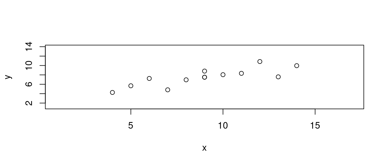
plot(df[c(index, OUTindex),],
     xlim = range(df[, "x"]) + c(-3, 3),
     ylim = range(df[, "y"]) + c(-3, 3),
     col = c(rep(1, length(index)), rep(2, length(OUTindex))))
# 繪製散佈圖。左右上下各加3個單位,方便大家觀察。
abline(m0, col = "blue")
abline(m1, col = "red")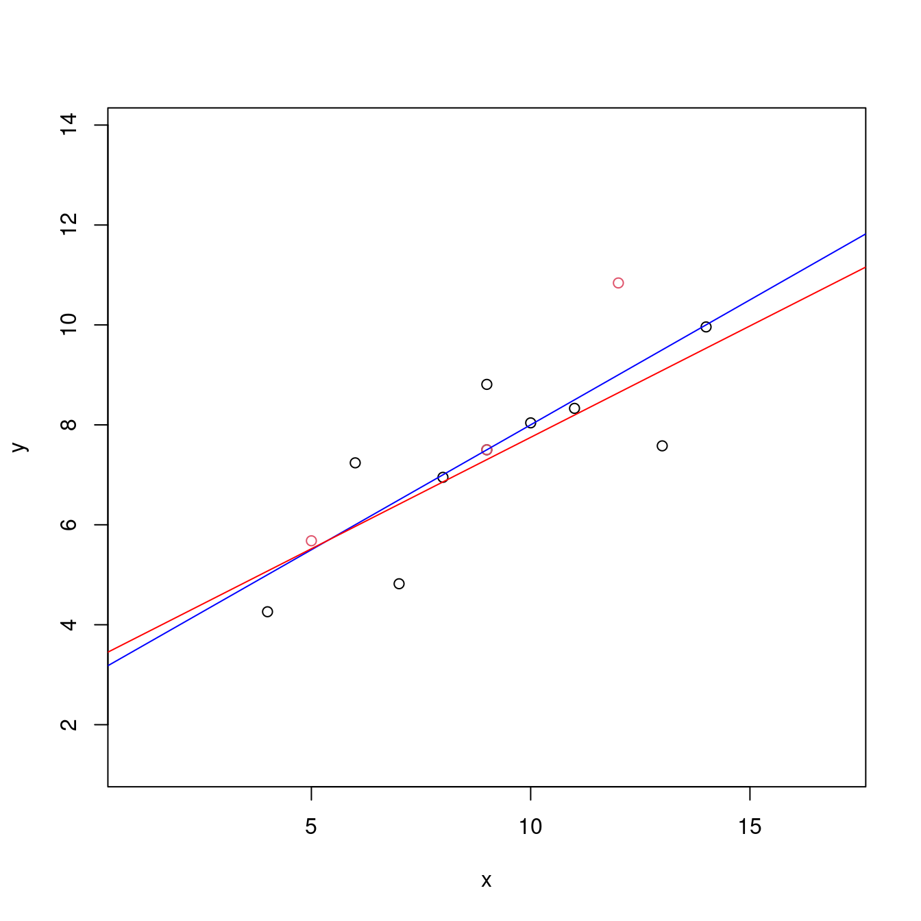
- 迴歸診斷圖。
par(mfrow = c(2, 2))
plot(m1)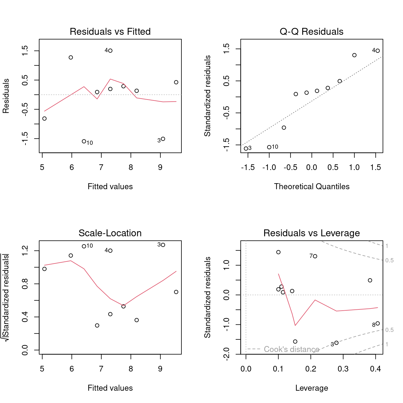
15.8.3 預測之外插法
df$x## [1] 10 8 13 9 11 14 6 4 12 7 5 9 9trainX <- sort(df$x)[1:floor(length(df$x)*0.80)]
trainX## [1] 4 5 6 7 8 9 9 9 10 11index <- which(df$x %in% trainX)
index## [1] 1 2 4 5 7 8 10 11 12 13OUTindex <- (1:dim(df)[1])[-index]
OUTindex## [1] 3 6 9train <- df[index,]
test <- df[-index,]
m2 <- lm(y ~ x, data = train)
m2##
## Call:
## lm(formula = y ~ x, data = train)
##
## Coefficients:
## (Intercept) x
## 2.5807 0.5554PREDtest <- predict(m2, test)
PREDtest## 3 6 9
## 9.801483 10.356926 9.246041SSPE <- sum((test$y - PREDtest)^2)
SSPE## [1] 7.633244SSE <- sum(m2$residuals^2)
SSE## [1] 6.547195SSE + SSPE## [1] 14.18044plot(df[c(index, OUTindex),],
xlim = range(df[, "x"]) + c(-3, 3),
ylim = range(df[, "y"]) + c(-3, 3),
col = c(rep(1, length(index)), rep(2, length(OUTindex))))
# 繪製散佈圖。左右上下各加3個單位,方便大家觀察。
abline(m0, col = "blue")
abline(m1, col = "red")
abline(m2, col = "green")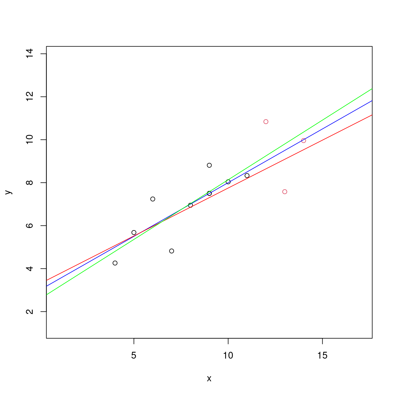
15.9 簡單線性迴歸分析可以是一種機器學習演算法嗎?
require(datasets) # 通常我們是這麼寫「library(datasets)」。
data("anscombe") # 載入。
anscombe # 呼叫它。
## x1 x2 x3 x4 y1 y2 y3 y4
## 1 10 10 10 8 8.04 9.14 7.46 6.58
## 2 8 8 8 8 6.95 8.14 6.77 5.76
## 3 13 13 13 8 7.58 8.74 12.74 7.71
## 4 9 9 9 8 8.81 8.77 7.11 8.84
## 5 11 11 11 8 8.33 9.26 7.81 8.47
## 6 14 14 14 8 9.96 8.10 8.84 7.04
## 7 6 6 6 8 7.24 6.13 6.08 5.25
## 8 4 4 4 19 4.26 3.10 5.39 12.50
## 9 12 12 12 8 10.84 9.13 8.15 5.56
## 10 7 7 7 8 4.82 7.26 6.42 7.91
## 11 5 5 5 8 5.68 4.74 5.73 6.89df <- anscombe[, c("x1", "y1")] # 取出「x1」跟「y1」,其中「1」代表第一組。
colnames(df) <- c("x", "y") # 劃掉其中的「1」。
df # 呼叫出來再一次檢視這一組數據集。## x y
## 1 10 8.04
## 2 8 6.95
## 3 13 7.58
## 4 9 8.81
## 5 11 8.33
## 6 14 9.96
## 7 6 7.24
## 8 4 4.26
## 9 12 10.84
## 10 7 4.82
## 11 5 5.68compCost <- function(X, y, par){
m <- length(y)
J <- sum((X%*%par - y)^2)/(2*m)
return(J)
}
X <- matrix(c(rep(1,dim(df)[1]), df$x),
dim(df)[1],
2,
byrow = FALSE)
X## [,1] [,2]
## [1,] 1 10
## [2,] 1 8
## [3,] 1 13
## [4,] 1 9
## [5,] 1 11
## [6,] 1 14
## [7,] 1 6
## [8,] 1 4
## [9,] 1 12
## [10,] 1 7
## [11,] 1 5y <- df$y
y## [1] 8.04 6.95 7.58 8.81 8.33 9.96 7.24 4.26 10.84 4.82 5.68theta <- c(0, 0)
theta## [1] 0 0optim(par = theta, fn = compCost, X = X, y = y, method = "BFGS")## $par
## [1] 2.9999312 0.5001067
##
## $value
## [1] 0.6255768
##
## $counts
## function gradient
## 16 8
##
## $convergence
## [1] 0
##
## $message
## NULLm0 <- lm(y ~ x, data = df)
summary(m0)##
## Call:
## lm(formula = y ~ x, data = df)
##
## Residuals:
## Min 1Q Median 3Q Max
## -1.92127 -0.45577 -0.04136 0.70941 1.83882
##
## Coefficients:
## Estimate Std. Error t value Pr(>|t|)
## (Intercept) 3.0001 1.1247 2.667 0.02573 *
## x 0.5001 0.1179 4.241 0.00217 **
## ---
## Signif. codes: 0 '***' 0.001 '**' 0.01 '*' 0.05 '.' 0.1 ' ' 1
##
## Residual standard error: 1.237 on 9 degrees of freedom
## Multiple R-squared: 0.6665, Adjusted R-squared: 0.6295
## F-statistic: 17.99 on 1 and 9 DF, p-value: 0.00217theta <- c(3, 0.5)
theta## [1] 3.0 0.5optim(par = theta, fn = compCost, X = X, y = y, method = "BFGS")## $par
## [1] 3.0000344 0.5000965
##
## $value
## [1] 0.6255768
##
## $counts
## function gradient
## 8 3
##
## $convergence
## [1] 0
##
## $message
## NULLcompCostLASSO <- function(X, y, par){
m <- length(y)
J <- sum((X%*%par - y)^2)/(2*m) + 0.01 * sum(par^2)
return(J)
}
theta <- c(0, 0)
theta
## [1] 0 0optim(par = theta, fn = compCostLASSO, X = X, y = y, method = "BFGS")## $par
## [1] 2.5464902 0.5448328
##
## $value
## [1] 0.7046972
##
## $counts
## function gradient
## 16 8
##
## $convergence
## [1] 0
##
## $message
## NULLcompCostRidge <- function(X, y, par){
m <- length(y)
J <- sum((X%*%par - y)^2)/(2*m) + 0.01 * sum(abs(par))
return(J)
}
theta <- c(0, 0)
theta## [1] 0 0optim(par = theta, fn = compCostRidge, X = X, y = y, method = "BFGS")## $par
## [1] 2.9179491 0.5081049
##
## $value
## [1] 0.6602086
##
## $counts
## function gradient
## 16 8
##
## $convergence
## [1] 0
##
## $message
## NULL15.9.1 當「最小平方法」變成「最大概似函數法」
作者小編先拷貝一份來自How to use optim in R的參考碼:
obs <- c(1,2,3,4,5,6,7,8,9,10,11,12,13,17,42,43)
freq <- c(1392,1711,914,468,306,192,96,56,35,17,15,6,2,2,1,1)
x <- rep(obs, freq)
plot(table(x), main = "Count data")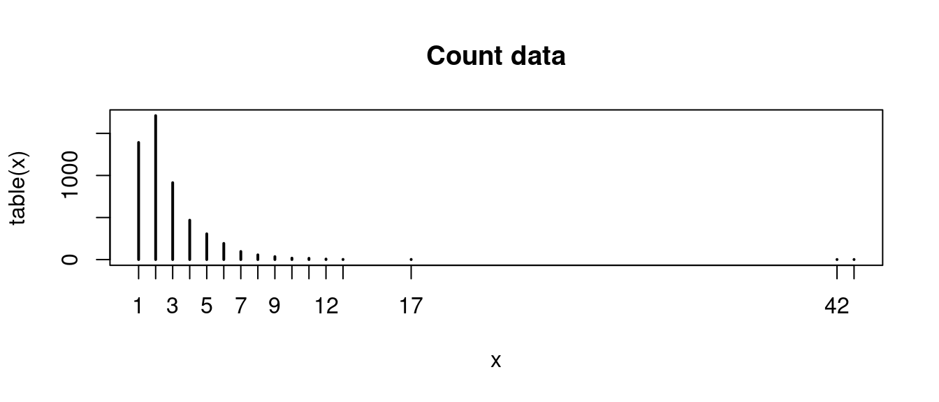
lklh.poisson <- function(x, lambda) {
 lambda^x/factorial(x) * exp(-lambda)
}

log.lklh.poisson <- function(x, lambda){
  -sum(x * log(lambda) - log(factorial(x)) - lambda)
}

optim(par = 2, log.lklh.poisson, x = x)
## Warning in optim(par = 2, log.lklh.poisson, x = x): 用 Nelder-Mead 方法來算一維最佳化不很可靠:
## 用"Brent"或直接用 optimize()## $par
## [1] 2.703516
##
## $value
## [1] 9966.067
##
## $counts
## function gradient
## 24 NA
##
## $convergence
## [1] 0
##
## $message
## NULLoptim(par = 2, fn = log.lklh.poisson, x = x,
method = "Brent",
lower = 2,
upper = 3)## $par
## [1] 2.703682
##
## $value
## [1] 9966.067
##
## $counts
## function gradient
## NA NA
##
## $convergence
## [1] 0
##
## $message
## NULLrequire(MASS)
fitdistr(x, "Poisson")## lambda
## 2.70368239
## (0.02277154)mean(x)## [1] 2.70368215.11 參考書
knitr::include_url("https://lgatto.github.io/IntroMachineLearningWithR/index.html")knitr::include_url("https://bradleyboehmke.github.io/HOML/")knitr::include_url("https://daviddalpiaz.github.io/r4sl/")…
15.12 專題參考文獻
knitr::include_url("https://machinelearningmastery.com/machine-learning-in-r-step-by-step/")- R的機器學習專欄
knitr::include_url("https://cran.r-project.org/web/views/MachineLearning.html")