Lesson 9 The bootstrap

In this lesson, you’ll learn an important practical tool for statistical inference on real data-analysis problems, called the bootstrap. Specifically, you’ll learn about:

the bootstrap sampling distribution.
bootstrap standard errors and confidence intervals.
how the bootstrap usually, but not always, works well.

A quick review

Let’s remind ourselves of where things stand. In the previous lesson, we learned about the core ideas of statistical inference. Specifically, we learned how the sampling distribution formalizes the concept of “statistical uncertainty” in terms of a thought experiment: what would happen if we could run the same analysis in many imaginary parallel universes, where in each parallel universe we experience a single realization of the same random data-generating process? Here’s the picture we saw in the last lesson, to illustrate this idea:

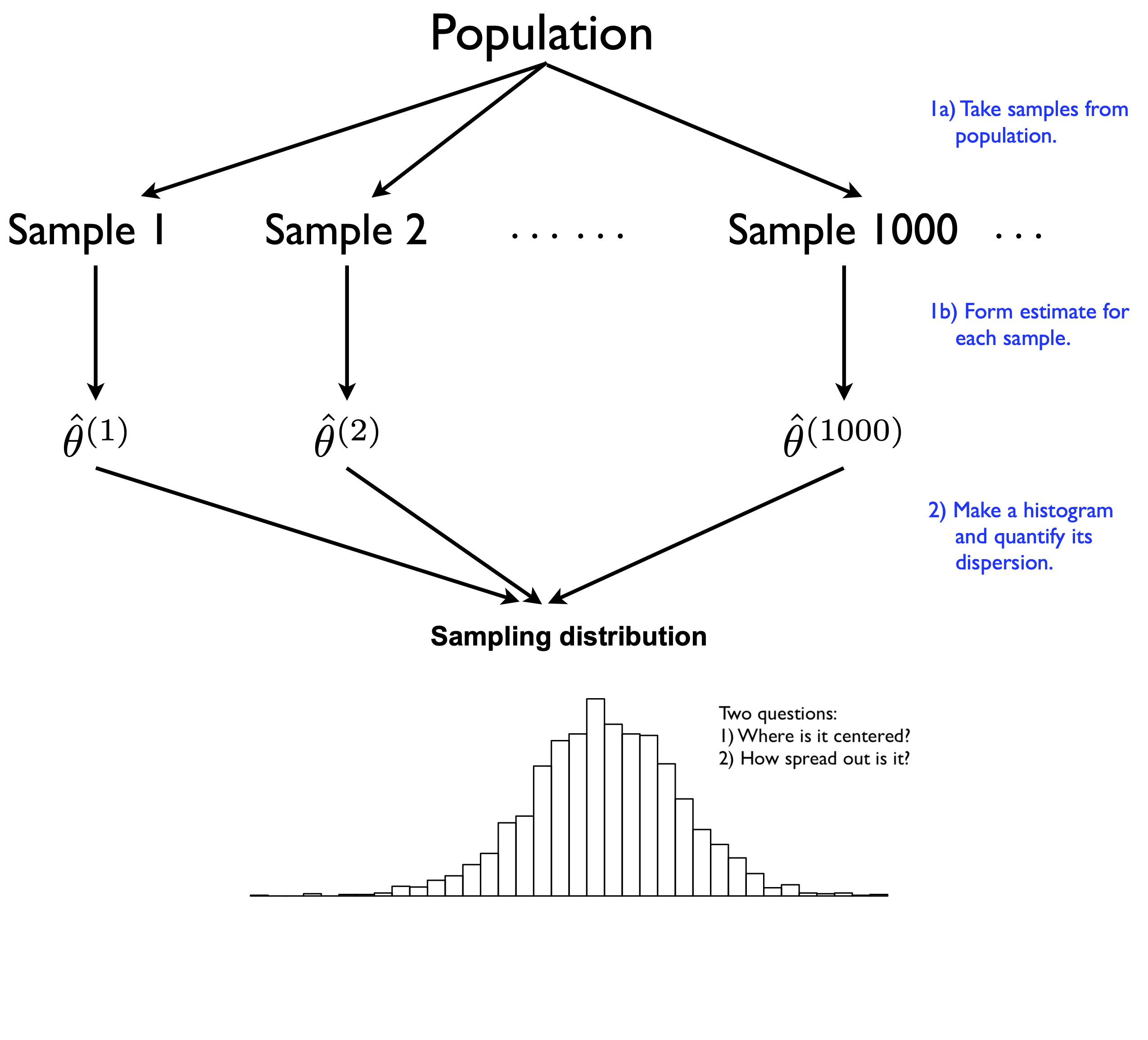
Figure 9.1: A review of the thought experiment behind a sampling distribution.

Of course, if you really could peer into all those parallel universes, each with its own sample from the same data-generating process, life would be easy. By examining all the estimates from all those different samples and seeing how much they differed from one another, you could calculate a standard error. You could then report a measure of uncertainty: “My estimate should be expected to err by about ____,” where you fill in the blank with the standard error you calculated.²⁷

In reality, however, we’re stuck with one sample. We therefore cannot ever know the actual sampling distribution of an estimator, for the same reason that we cannot peer into all those other lives we might have lived, but didn’t:

Two roads diverged in a yellow wood,
And sorry I could not travel both
And be one traveler, long I stood
And looked down one as far as I could
To where it bent in the undergrowth.
– Robert Frost, The Road Not Taken, 1916

Quantifying our uncertainty would seem to require knowing all the roads not taken—an impossible task.

So in light of that you might ask, rather fairly: what the hell have we been doing this whole time? Here’s what. Surprisingly, we actually can come quite close to performing the impossible. There are two ways of feasibly constructing something like the histogram in Figure 9.1, thereby approximating an estimator’s sampling distribution—all without ever taking repeated samples from the true data-generating process.

Resampling: that is, by pretending that the sample itself represents the population, which allows one to approximate the effect of sampling variability by resampling from the sample.
Mathematical approximations: that is, by recognizing that the forces of randomness obey certain mathematical regularities, and by drawing approximate conclusions about these regularities using probability theory.

In this lesson, we’ll discuss the resampling approach at length, covering the mathematical approach in a later lesson and at a fairly coarse level of detail (i.e. with almost no math involved).

9.1 The bootstrap sampling distribution

At the core of the resampling approach to statistical inference lies a simple idea. Most of the time, we can’t feasibly take repeated samples from the same random process that generated our data, to see how our estimate changes from one sample to the next. But we can repeatedly take resamples from the sample itself, and apply our estimator afresh to each notional sample. The variability of the estimates across all these resamples can be then used to approximate our estimator’s true sampling distribution.

This process—pretending that our sample represents some notional population, and taking repeated samples of size $N$ with replacement from our original sample of size $N$—is called bootstrap resampling, or just bootstrapping.²⁸

Why would this work? Remember that uncertainty arises from the randomness inherent to our data-generating process (be it sampling variability, measurement error, whatever). So if we can approximately simulate this randomness, then we can approximately quantify our uncertainty. That’s the goal of bootstrapping: to approximate the randomness inherent to data-generating process, so that we can simulate the core thought experiment of statistical inference.

Here’s what bootstrapping looks like in a picture.

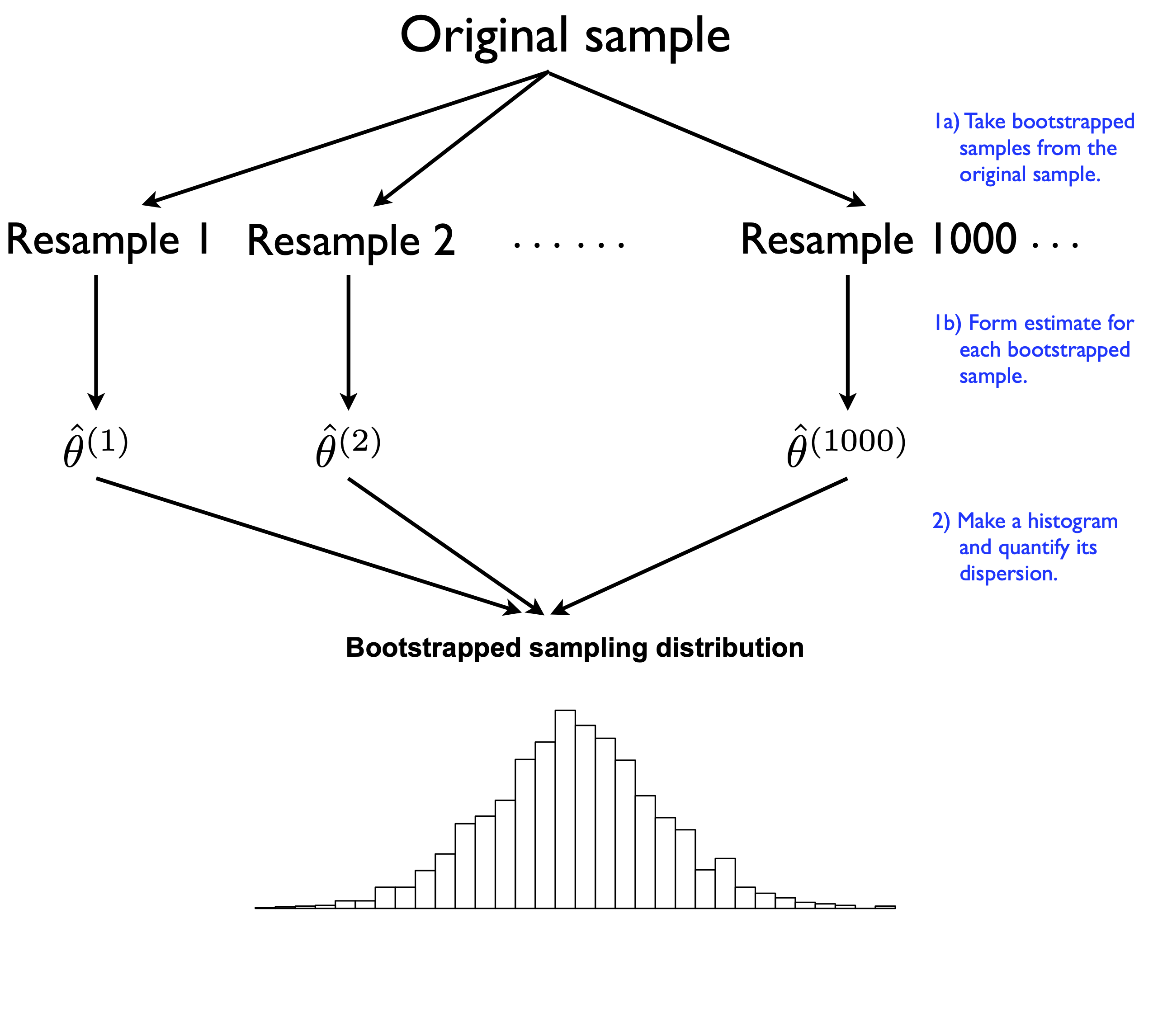
Figure 9.2: A stylized depiction of a bootstrap sampling distribution of an estimator.

Each block of $N$ resampled data points is called a “bootstrap sample.” To bootstrap, we write a computer program that repeatedly resamples our original sample and recomputes our estimate for each bootstrap sample. As we’ll see shortly, R makes a non-issue of the calculational tedium involved in actually doing this.

There are two key properties of bootstrapping that make this seemingly crazy idea actually work. First, each bootstrap sample must be of the same size (N) as the original sample. Remember, we have to approximate the randomness in our data-generating process, and the sample size is an absolutely fundamental part of that process. If we take bootstrap samples of size N/2, or N-1, or anything else other than N, we are simulating the “wrong” data-generating process.

Second, each bootstrap sample must be taken with replacement from the original sample. The intuition here is that each bootstrap sample will have its own random pattern of duplicates and omissions compared with the original sample, creating synthetic sampling variability that approximates true sampling variability.

To understand sampling with replacement, imagine a lottery drawing, where there’s a big bucket with numbered balls in it. We choose 6 numbers from the bucket. After we choose a ball, we could do one of two things: 1) put the ball to the side, or 2) record the number on the ball and then throw it back into the bucket. If you set a ball aside after it’s been chosen, it can be chosen only once; this is sampling without replacement, and it’s what happens in a real lottery. But if instead you put the ball back into the bucket, it has a some small chance of being chosen again, and therefore being represented more than once in the final set of 6 lottery numbers. This is sampling with replacement, and it’s what we do when we bootstrap.

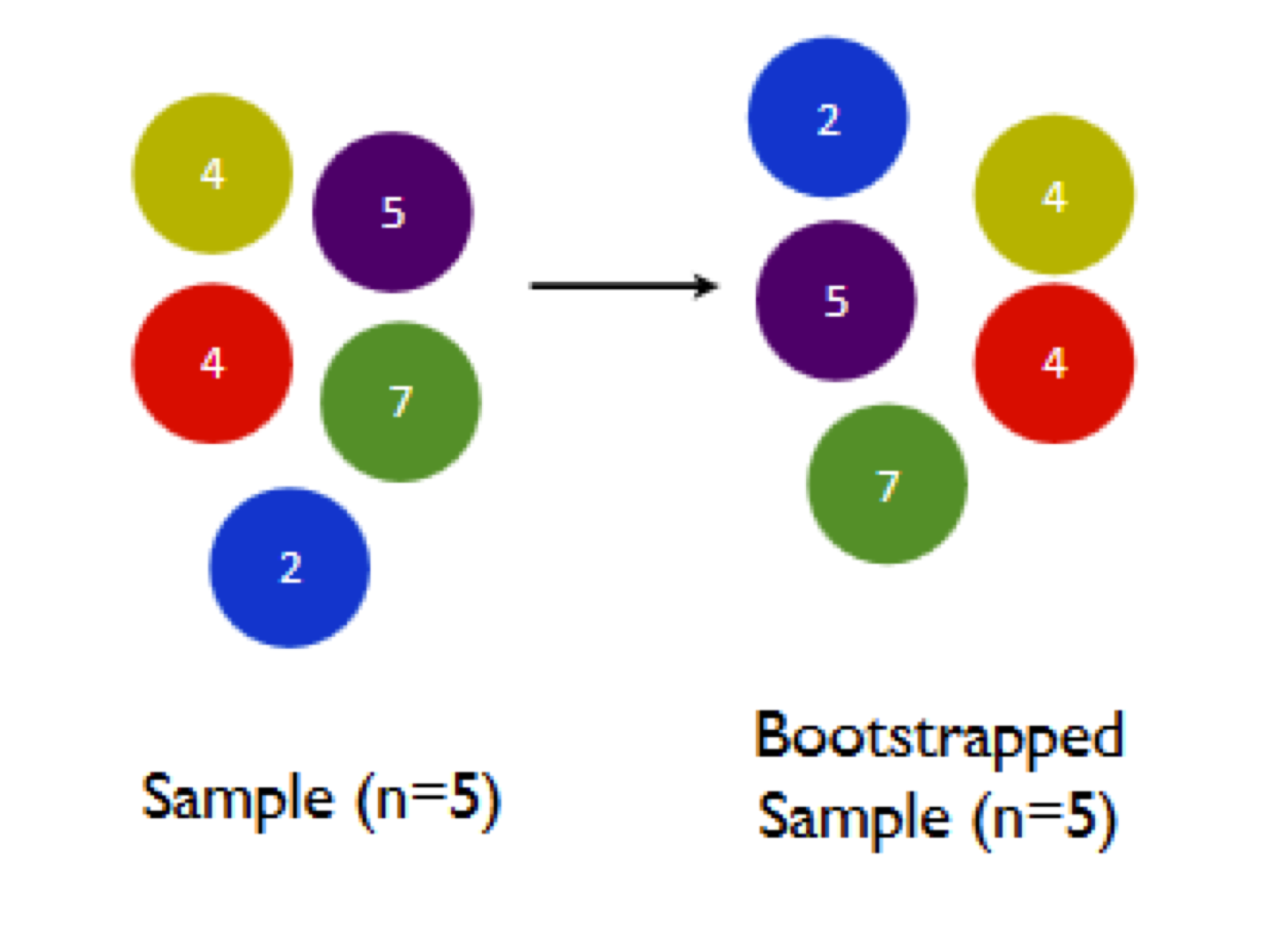
Let’s see how this “sampling with replacement” process works in the context of bootstrapping, and why it’s important. In the cartoon below, the left panel shows a hypothetical sample of size N=5, while the right panel shows a bootstrap sample from this original sample.

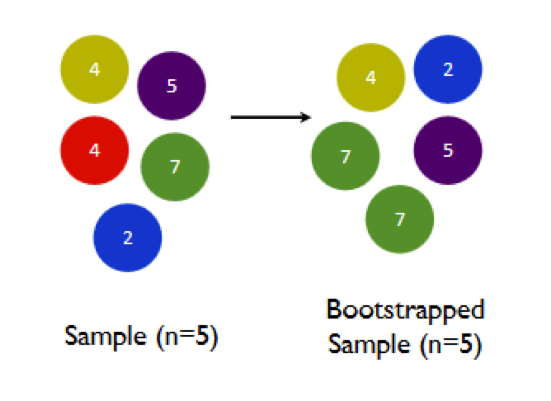
Notice the two key properties of our bootstrap sample: (1) the bootstrap sample is the same size (N=5) as the original sample; and (2) the bootstrap sample was taken with replacement, and therefore has a random pattern of duplicates and omissions when compared with the original sample. Specifically, the red 4 has been omitted entirely, while the green 7 has been chosen twice.

Why does this matter? Well, let’s see what happens when we calculate the sample mean of the bootstrap sample, versus the original sample:

sample mean of original sample: $(4 + 5 + 4 + 7 + 2)/5 = 4.4$
sample mean of bootstrap sample: $(4 + 2 + 7 + 5 + 7)/5 = 5$

And this is the core fact to notice: when we compute a summary statistic for the bootstrap sample, we won’t necessarily get the same answer as we did for the original sample.

Let’s see another bootstrap sample, to emphasize this variability:

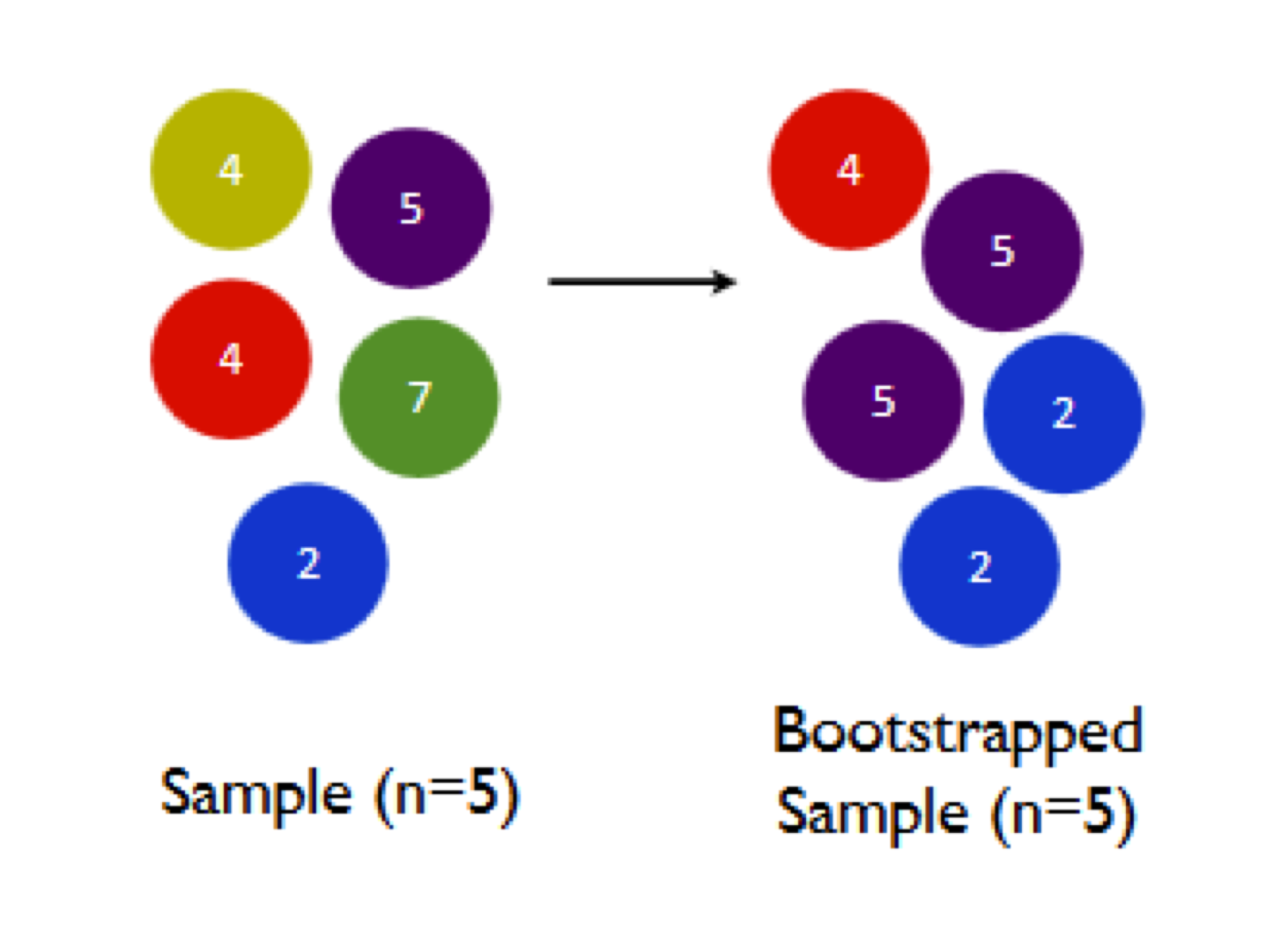
Now the orange 4 and the green 7 have been omitted, while both the purple 5 and blue 2 have been duplicated. As a result, we get a different sample mean:

sample mean of original sample: $(4 + 5 + 4 + 7 + 2)/5 = 4.4$
sample mean of 1st bootstrap sample: $(4 + 2 + 7 + 5 + 7)/5 = 5$
sample mean of 2nd bootstrap sample: $(4 + 5 + 5 + 2 + 2)/5 = 3.6$

Let’s see one final bootstrap sample, just to fix our intuition for what’s going on:

A third different pattern of duplicates and omissions, and a third different bootstrap sample mean. By sheer luck, this one happens to be the same as the mean of the original sample:

sample mean of original sample: $(4 + 5 + 4 + 7 + 2)/5 = 4.4$
sample mean of 1st bootstrap sample: $(4 + 2 + 7 + 5 + 7)/5 = 5$
sample mean of 2nd bootstrap sample: $(2 + 4 + 5 + 4 + 7)/5 = 3.6$
sample mean of 3rd bootstrap sample: $(2 + 4 + 5 + 4 + 7)/5 = 4.4$

This is the core mechanism by which bootstrapping works: resampling creates synthetic variability in our statistical summaries, in a way that’s design to approximate true sampling variability. If we repeat this process thousands of times, some summaries will be too high, some will be too low, and a few will be just right when compared with the answer from the original sample. The point is, the bootstrap summaries differ from one another—and the amount by which they differ from one another provides us a quantitative measure of our statistical uncertainty.

And that’s the basic idea:

You’re certain if your results are repeatable under different samples from the same random data-generating process.
Bootstrapping lets you measure the repeatability of your results, by approximating the process of sampling randomly from the wider population.

The core assumption of the bootstrap

The core assumption of the bootstrap is that the randomness in your data, and therefore the statistical uncertainty in your answer, arises from the process of sampling. That is, the bootstrap implicitly assumes that your samples can be construed as random samples from some wider reference population. While the bootstrap isn’t explicitly designed for anything else, it’s actually provides a pretty good approximation for other common forms of randomness as well.²⁹ These include:

experimental randomization.
measurement error.
intrinsic variability of some natural process (e.g. your heart rate).

So while we’ll motivate the bootstrap as an approximation to random sampling, we’ll actually use it in a broader set of situations, where random sampling isn’t necessarily the reason we face statistical uncertainty about our answers.³⁰

9.2 Bootstrapping summaries

Let’s bootstrap! Please load the tidyverse and mosaic libraries:

library(tidyverse)
library(mosaic)

Please also download and import the data in NHANES_sleep.csv. This file contains a sliver of data from the National Health and Nutrition Examination Survey, known as NHANES. NHANES is a major national survey run by the US Centers for Disease Control and Prevention (CDC). Per the CDC, it is “designed to assess the health and nutritional status of adults and children in the United States.” It is intended to be a nationally representative survey whose results can generalized to the broader American population—and indeed, it is basically as good as surveys ever get in that regard, at least outside the pages of a statistics textbook. Moreover, NHANES is unusually comprehensive as far as health surveys go, in that it combines both interviews and physical exams.

Here, we’ll be looking at a subset of 1,991 survey participants from the 2011-12 version of the survey, focused on a few questions surrounding sleep and depression. (The full data set has a lot more information than what you’ll see in this file.) The NHANES_sleep file contains information on people’s gender, age, self-reported race/ethnicity, and home ownership status. It also has a few pieces of health information: 1) the self-reported number of hours each study participant usually gets at night on weekdays or workdays; 2) whether the respondent has smoked 100 or more cigarettes in their life (yes or no); and 3) the self-reported frequency of days per month where the participant felt down, depressed or hopeless, where the options are “None,” “Several,” “Majority” (more than half the days), or “Almost All.”

The first five lines of the data file look like this.

head(NHANES_sleep, 5)

##   SleepHrsNight Gender Age Race_Ethnicity HomeOwn Depressed Smoke100
## 1             4 female  56          Black     Own      None      Yes
## 2             7   male  34     White (NH)    Rent      None       No
## 3             7   male  27     White (NH)    Rent      None       No
## 4             9   male  50     White (NH)     Own      None       No
## 5             6   male  80          Black    Rent      None       No

Example 1: sample mean

The first question we’ll address is: how well are Americans sleeping, on average? Our first pass here might be to plot the data distribution for the SleepHrsNight variable in a histogram:

ggplot(NHANES_sleep) + 
  geom_histogram(aes(x = SleepHrsNight), binwidth=1)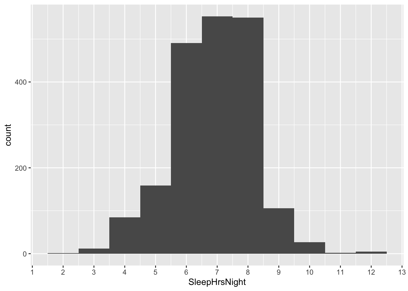

So it looks like the sample mean is somewhere around 7 hours per night, but with a lot of variation around that mean: some people sleep a lot more than 7 hours, and some people sleep a lot less. To calculate the mean a bit more precisely, we’ll use one of the “shortcut” functions that we learned in the section on Summary shortcuts, a few lessons back, to calculate the average number of hours per night that our survey respondents said they slept:

mean(~SleepHrsNight, data=NHANES_sleep)

## [1] 6.878955

According to the survey, it’s 6.88 hours per night, on average. But remember, this is just a survey—a very well-designed survey, but a survey nonetheless. We clearly have some uncertainty in generalizing this number to the wider American population.

How much? To get a rough idea, let’s take a single bootstrap sample to simulate the randomness of our data-generating process, like this:

NHANES_sleep_bootstrap = mosaic::resample(NHANES_sleep)
mean(~SleepHrsNight, data=NHANES_sleep_bootstrap)

## [1] 6.833385

Taking each line in turn:

the first line says to resample the NHANES_sleep data set, and to store the result in an object called NHANES_sleep_bootstrap. Why mosaic::resample rather than just resample? Because resample is a common name used in multiple R packages. By adding mosaic:: in front of resample, we clarify to R that we want to use the version of that function defined in the mosaic library.³¹ (By default, mosaic’s resample function takes a sample with replacement of the same size as your original sample, which are the two key requirements of bootstrapping.)
the second line says to calculate the mean of the SleepHrsNight variable for the bootstrap sample (i.e. not for the original sample).

The result is about 6.83 hours, on average. This differs from 6.88, the mean of the original sample, by about 0.05 hours, or 3 minutes. Remember, this difference represents a sampling error. (Or more precisely, it represents a bootstrap sampling error, which is an approximation to an actual sampling error.) So we’ve already learned something useful: our survey result of 6.88 hours per night could easily differ from the true population average by 3 minutes, just because of the uncertainty inherent to sampling. We know this is possible because we saw a 3-minute error happen right before our eyes!

I don’t know about you, but my reaction to that number is that 3 minutes seems like a pretty small error, at least compared with an average sleep of nearly 7 hours. It seems to suggest that our statistical uncertainty is pretty small—in other words, that we know the average sleep time of the American population in 2011-12 pretty precisely based on the NHANES survey.

But of course, that error of 3 minutes, or 0.05 hours, was based on just a single bootstrap sample. Was 3 minutes a typical sampling error? Or might it instead have been an abnormally small (or abnormally large) sampling error?

Let’s run 10,000 bootstrap samples to find out. It turns out that we can do this in a single line of R code that combines do with resample. (Remember do from our prior lesson on Sampling distributions.) The following line might take ten seconds or so to execute on your machine, so be patient:

boot_sleep = do(10000)*mean(~SleepHrsNight, data=mosaic::resample(NHANES_sleep))

This statement says to: 1) create 10,000 bootstrap samples from the original NHANES_sleep data frame, and 2) for each bootstrap sample, recompute the mean of the SleepHrsNight variable. We store the resulting set of 10,000 sample means in an object called boot_sleep.

What does this boot_sleep object look like? Let’s examine the first several lines:

head(boot_sleep)

##       mean
## 1 6.844299
## 2 6.832245
## 3 6.897539
## 4 6.918634
## 5 6.873430
## 6 6.853340

We see a single column called mean, with each entry representing the mean for a single bootstrap sample. Let’s make a histogram of these 10,000 different means:

ggplot(boot_sleep) + 
  geom_histogram(aes(x=mean))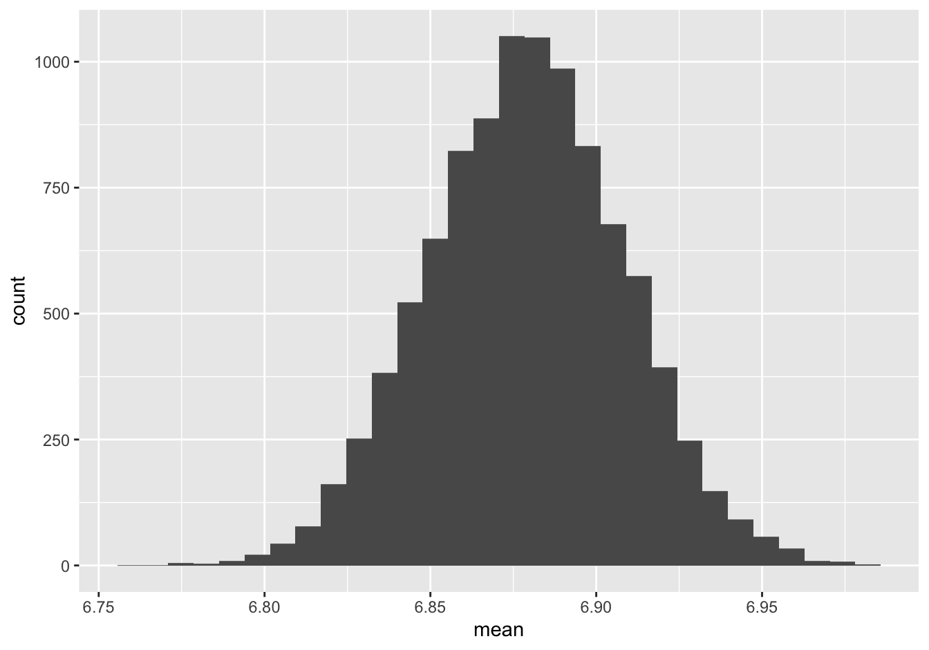

This histogram represents our bootstrap sampling distribution, which is designed to approximate the true sampling distribution we talked about in the previous lesson.

Bootstrap standard errors and confidence intervals

So now what do we do with this sampling distribution? The answer is: we ask the same two questions we’re supposed to ask about any sampling distribution!

First, where is it centered? It looks to be centered around 6.88 hours of sleep, which you’ll recall is the sample mean from our original sample. This makes sense, since by the logic of bootstrapping, the original sample is our surrogate for the population. This is reassuring: it’s telling us that the sampling process seems to be getting the “right” answer on average. Of course, we don’t know the right answer for the population, but we do know the right answer for our original sample. And this “original sample answer” is exactly what we’d hope to see from the average of the bootstrap samples. The logic here is, roughly: if sampling from the original sample gets the original sample’s answer right, on average, then we feel reassured that sampling from the population will get the population’s answer right, on average (even if we don’t know what the population answer is).

Second, how spread out is the sampling distribution? Let’s calculate a standard error:

boot_sleep %>%
  summarize(std_err_sleep = sd(mean))

##   std_err_sleep
## 1    0.02945353

So it looks like a “typical” sampling error is about 0.03 hours, or roughly 2 minutes. We can conclude that we know the average sleep time of the American population pretty precisely based on the NHANES survey: it’s 6.88 hours, up to an error of about 0.03 hours, or two minutes. In other words, if we actually could ask everyone in America, we feel pretty confident that the average of all their answers would fall somewhere in the range 6.88 $\pm$ 0.03 hours.

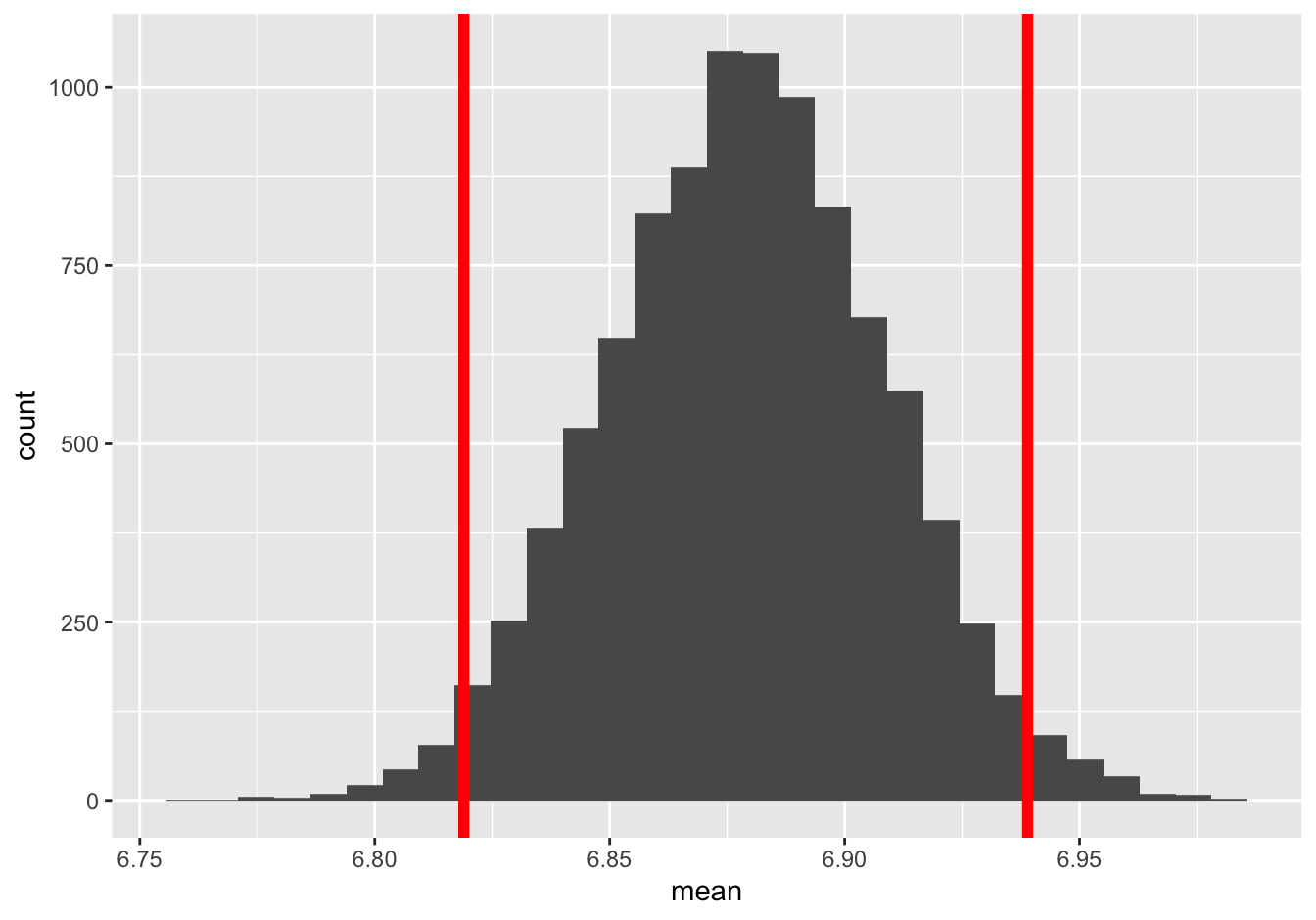
We said we’re “pretty confident” that the answer is 6.88 $\pm$ 0.03, but “pretty” confident is a bit of a weasel word. Just how confident are we? To answer, let’s examine the histogram again, and ask what proportion of sampling errors seem to be 0.03 or less.

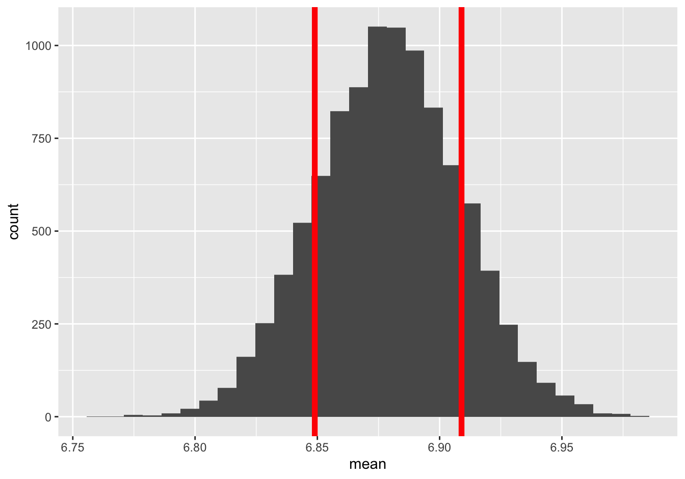
The area between the red lines corresponds to bootstrap sampling errors of 0.03 or less (that is, within one standard error of the middle of the sampling distribution). Just eyeballing it, I’d say that roughly two-thirds of the bootstrap means fall in this window. Therefore, again just eyeballing it, I’d say that I’m about 65-70% confident that the average American’s sleep time falls in the interval 6.88 $\pm$ 0.03 hours.

Of course, we can use summarize to check, if we want to be sure:

boot_sleep %>%
  summarize(prob_within_1se = sum(mean > 6.88 - 0.03 & mean < 6.88 + 0.03))

##   prob_within_1se
## 1            6825

That’s 6,825 out of 10,000, or 68%. Therefore, we’d refer to the interval 6.88 $\pm$ 0.03 as a 68% confidence interval. In other words: our best guess is 6.88, and we’re 68% confident that our guess is within 0.03 hours of the truth either way. (Of course, you might get a slightly different number, like 67% or 69%, due to Monte Carlo variability.)

Now, you might object to one thing here, purely on the grounds of sociability: normal people don’t walk around saying things like “I’m 68% confident that so and so is true.” I mean, 68%? It just isn’t done. Of course there’s nothing wrong with 68% as a confidence level; it’s just that most people will regard it as a weirdly specific number, and possibly regard you as a weirdly specific individual, if you say it out loud. Moreover, even if you’re immune to such conformist pressure, you might also legitimately object that 68% is simply too low, that serious people will not tolerate such wishy-washiness, and that you therefore want to express your conclusions with a higher level of confidence.

So how does 95% sound? It’s a big, round number, which people seem to like—and moreover, it’s also a number that falls just enough short of 100% so that you won’t look like a complete idiot if you end up being wrong. Perhaps for these reasons, 95% is a conventional choice of confidence level that won’t raise any eyebrows. So let’s roll with it, using the confint function:

confint(boot_sleep, level=0.95)

##   name    lower    upper level     method estimate
## 1 mean 6.821698 6.937217  0.95 percentile  6.92667

This is a 95% confidence interval for the average weekday sleep time of the American population. It says that our best guess is about 6.88 hours per night, and that we’re 95% confident that the right answer is somewhere between 6.82 and 6.94, or equivalently, 6.88 $\pm$ 0.06.

It might help to see this 95% confidence interval superimposed on the bootstrap sampling distribution. Here it is:

It’s basically like taking a little axe and chopping off 2.5% of the bootstrap sampling distribution in either tail, leaving the middle 95% as your confidence interval.

You might notice that this 95% interval ends up covering two standard errors, or 0.06 hours, to either side of your sample estimate of 6.88. This specific numerical correspondence (68% for 1 standard error, 95% for 2) happens frequently enough to warrant a rule of thumb:

Confidence interval rule of thumb: a 95% confidence interval tends to be about two standard errors to either side of your best guess. A 68% confidence interval tends to be about one standard error to either side of your best guess.

But when in doubt, you can always use confint at whatever level you choose.

The biggest bootstrapping gotcha

Let’s talk about the biggest “gotcha” in bootstrapping. It concerns the following fact: that the data distribution of some variable (like SleepHrsNight) and the sampling distribution for the mean of that variable are two fundamentally different things. The biggest bootstrapping “gotcha” turns on conflating the two.

In fact, I’ve learned over the years that if the students in my data science class are crushing it, and if I fear that the dean will start to yell at me about grade inflation more loudly than the students will yell at me about their B+, then I can always buy myself some breathing room by throwing in a question along these lines on the midterm. Mean, you say? Not at all; it’s not like this is a trick question. You cannot possibly fall for this particular “gotcha” unless you exhibit an absolutely fundamental misunderstanding about the bootstrap, and about the sampling distribution more generally.

Let’s see an example “gotcha.” The setup here is going to feel familiar, because it’s precisely the NHANES survey we’ve already been talking about. Suppose we have a random sample of 1,991 Americans, and we ask each of them how many hours of sleep they get per night. We calculate the average as 6.88 hours, and then we bootstrap the sample in order to form a bootstrap sampling distribution:

boot_sleep = do(10000)*mean(~SleepHrsNight, data=mosaic::resample(NHANES_sleep))

We examine the sampling distribution and compute a 95% confidence interval, like this:

ggplot(boot_sleep) + 
  geom_histogram(aes(x=mean))

confint(boot_sleep, level = 0.95)

##   name    lower    upper level     method estimate
## 1 mean 6.821698 6.937217  0.95 percentile 6.892014

So here’s the question. I strongly suggest that, as a self-diagnostic, you answer for yourself before you click on the spoiler alert.

True or false: this histogram, and the associated confidence interval, tell us that about 95% of all Americans sleep somewhere between 6.82 and 6.94 hours on an average night (rounded to two decimal places).

FALSE, FALSE, 10,000 times FALSE. Hey, look, I’m not disappointed in you or anything if you thought the answer was “true.” It’s a very common misunderstanding and there’s no shame in it. But if you’re one of those folks who thought this statement was true, I will level with you: there’s a very good chance that you need to go back to the beginning of the lesson on Statistical uncertainty and start over from there, proceeding very carefully until you reach this point again. In the lessons to come, almost nothing is going to hang together for you until you understand why “true” is the wrong answer—or, even better, how you could amend the statement so that it actually is true.

So why is this statement false? The reason is that the sampling distribution isn’t telling us about variation in individual Americans’ sleep habits. That’s what the data distribution tells us. Instead, the sampling distribution of the mean is telling about the level of precision with which we can estimate the mean of the population, based on the mean of the data distribution. The population mean collapses a huge amount of individual variation into a single number. So a correct statement would be: “This histogram, and the associated confidence interval, tell us that we can be 95% confident based on this sample that the population average sleep time is between 6.82 and 6.94 hours per night (rounded to two decimal places).”

To emphasize the difference between the data distribution and the sampling distribution, let’s actually look at the data distribution once again. This is the same histogram we saw at the very beginning of the NHANES example. It is the distribution of SleepHrsNight among all 1,991 survey respondents:

ggplot(NHANES_sleep) + 
  geom_histogram(aes(x = SleepHrsNight), binwidth=1)

Look how much wider the data distribution is than the sampling distribution. Clearly it is not true that 95% of all Americans sleep between 6.82 and 6.94 hours per night. In fact, such a statement is wildly false. Just eyeballing the histogram, a more reasonable statement might be that about 95% of all Americans sleep between 4 and 9 hours per night. There’s a huge amount of variation around the population mean.

What is true, however, is that this sample has allowed us to estimate this population mean quite precisely: it’s about 6.88 $\pm$ 0.06 hours per night, with 95% confidence. That’s our statistical uncertainty, and that’s what the sampling distribution is telling us.

The moral of the story is: don’t fall for the gotcha!

The data distribution of SleepHrsNight is real. You can plot it. You can see it. Variation around the mean of that distribution represents real things that happened to real people.
The sampling distribution of the mean of SleepHrsNight is something fundamentally different. It is, in the most literal sense of the word, imaginary. It’s a distribution of a bunch of imaginary means of imaginary answers from imaginary surveys about people’s sleep. For all that, however, this distribution is still really useful; it represents the results of a thought experiment about what we happen if we could take many different samples, whose variation can tell us about the precision of the mean from our sample.
The whole point of this lesson is that we can’t feasibly run that real thought experiment, so we run an approximate version of that thought experiment via the bootstrap.

Example 2: sample proportion

Let’s see a second example of the bootstrap in action. The next question we’ll address is: how frequent are feelings of depression among the American population? We’ll look at this using the variable Depressed, which is the self-reported frequency of days per month where a participant felt down, depressed or hopeless. The options are “None,” “Several,” “Majority” (more than half the days), or “Almost All.”

To keep the analysis simple, we’ll define a new variable called DepressedAny that encodes whether a participant’s response to this question was anything other than None:

NHANES_sleep = NHANES_sleep %>%
  mutate(DepressedAny = ifelse(Depressed != "None", yes=TRUE, no=FALSE))

Inside the ifelse statement, the != means “is not equal to.” So this statement encodes the DepressedAny variable as TRUE if that participant’s answer was anything other than None, and as FALSE otherwise.

Now let’s use the “shortcut” function that we learned in the section on Summary shortcuts, a few lessons back, to calculate the proportion of those in our survey who reported any depression:

prop(~DepressedAny, data=NHANES_sleep)

## prop_TRUE 
## 0.2034154

So about 20% of the sample. Mental health professionals are often telling us that depression is much more common than many people realize; here’s the evidence for you right here.

How precisely does this survey result characterize the frequency of depression among all Americans? Let’s bootstrap the sample to get a sense of our statistical uncertainty. This code might take ten seconds or so to run:

boot_depression = do(10000)*prop(~DepressedAny, data=mosaic::resample(NHANES_sleep))

This statement says to: 1) create 10,000 bootstrap samples from the original NHANES_sleep data frame, and 2) for each bootstrap sample, recompute the proportion of those for which the DepressedAny variable is equal to TRUE. We store the resulting set of 10,000 bootstrapped proportions in an object called boot_depression.

The first six lines of this object look as follows:

head(boot_depression)

##   prop_TRUE
## 1 0.1993973
## 2 0.1943747
## 3 0.1893521
## 4 0.2114515
## 5 0.1993973
## 6 0.2044199

There’s a single column called prop_TRUE, with each entry representing the proportion calculated from a single bootstrap sample. We can now examine this sampling distribution and compute a 95% confidence interval, like this:

ggplot(boot_depression) + 
  geom_histogram(aes(x=prop_TRUE))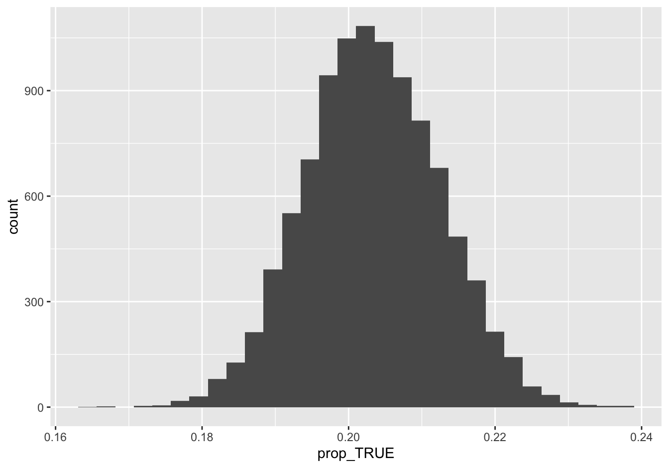

confint(boot_depression, level = 0.95)

##        name     lower     upper level     method  estimate
## 1 prop_TRUE 0.1854993 0.2214967  0.95 percentile 0.2034154

So our best guess is that 20.3% of Americans feel depressed at least some of the time. Moreover, based on the sample, we’re 95% confident that the true population proportion is somewhere between 18.5% and 22.1%. That interval represents our statistical uncertainty.

Another gotcha

Let’s once again take care to distinguish this confidence interval from the data distribution, via a second “gotcha.”

True or false: this histogram, and the associated confidence interval, tell us that about 95% of all Americans experience depression on somewhere between 18.5% and 22.1% of their days.

FALSE again. The variability in the data distribution is much, much wider than this. Some Americans experience depression every day. Some Americans experience depression never, or nearly never. This interval simply isn’t telling us about the variability in individual Americans’ experiences of depression. Rather, it is characterizing how precisely our sample has allowed us to estimate the population average frequency of Americans that experience any depressive days at all (our estimand).

9.3 Bootstrapping differences

What if we wanted to go one lever deeper with our data, by looking at specific subgroups? For example, we might ask how sleep or depression varies by gender. Or maybe how sleep varies among those with and without depression. We’ve already learned how to calculate summary statistics like means and proportions by group; now, with the bootstrap, we can also measure our statistical uncertainty about group differences.

Example 1: sleep hours by gender

Let’s take the case of average sleeping hours for males and females. Using one of our by-now-familiar “summary shortcuts,” we can calculate this in a single line of code, using mean:

mean(SleepHrsNight ~ Gender, data=NHANES_sleep)

##   female     male 
## 6.996954 6.763419

It looks like females sleep a bit longer than males, on average. If we just cared about that difference, we could use diffmean:

diffmean(SleepHrsNight ~ Gender, data=NHANES_sleep)

##   diffmean 
## -0.2335348

So among survey respondents, women sleep around 0.23 hours (14 minutes) longer per night than males, on average.

But what about statistical uncertainty? That is, how precisely can this difference for our sample characterize the corresponding difference for the wider American population? Let’s bootstrap our sample to find out:

boot_sleep_gender = do(10000)*diffmean(SleepHrsNight ~ Gender, data=mosaic::resample(NHANES_sleep))

This statement says to: 1) create 10,000 bootstrap samples from the original NHANES_sleep data frame, and 2) for each bootstrap sample, recompute the difference in the means of the SleepHrsNight variable between males and females. We store the resulting set of 10,000 bootstrapped differences in an object called boot_sleep_gender.

The resulting object has a single column called diffmean, with each entry representing the difference of means for a single bootstrap sample:

head(boot_sleep_gender)

##     diffmean
## 1 -0.1697103
## 2 -0.2828213
## 3 -0.4130471
## 4 -0.1896541
## 5 -0.4341876
## 6 -0.1945662

Let’s visualize this sampling distribution in a histogram, and then use it to create a confidence interval:

ggplot(boot_sleep_gender) + 
  geom_histogram(aes(x=diffmean))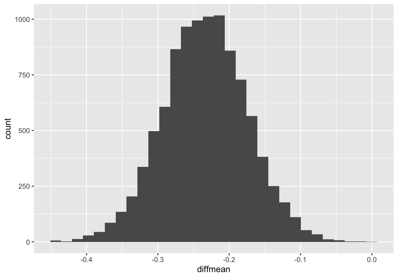

confint(boot_sleep_gender, level = 0.95)

##       name      lower      upper level     method   estimate
## 1 diffmean -0.3486014 -0.1171517  0.95 percentile -0.2335348

Based on this survey, we can say with 95% confidence that females get a bit more sleep than males, on average, with a difference in means of somewhere between 0.12 and 0.35 hours (7-21 minutes).

You’ll notice that this confidence interval rules out a difference of zero. We therefore say that the difference is statistically significant, i.e. nonzero up to a specified level of statistical uncertainty.

Definition 9.1 An estimate is said to be statistically significant at some specified level $\alpha$ if a confidence interval at level $1-\alpha$ for that estimate does not contain zero.

Somewhat confusingly, the convention is to report statistical significance as the opposite of confidence. So here, we’d say that the difference in average sleep time between males and females is statistically significant at the 5% (0.05) level, because a 95% (0.95) confidence interval for that difference fails to contain zero.

One last gotcha

Remember, this confidence interval of (-0.35, -0.12) is a claim about the difference between two population averages, one for males and one for females. It’s not a claim about individual males and females. So, for example, here’s one last “gotcha”:

True or false: this histogram, and the associated confidence interval, tell us that if we randomly sampled one male and one female from the population, we’re 95% confident that the female would sleep between 0.12 and 0.35 hours longer than the male.

FALSE. Again, the variability in the data distribution is much, much wider than this. Some males sleep 9 or 10 hours per night; some females sleep 4 or 5 hours per night. The confidence interval just isn’t telling us about the individual-level differences. Rather, it is characterizing how precisely our sample has allowed us to know the true value of our estimand: the difference between the average sleep time of all males living in America and the average sleep time of all females living in America.

To help you visualize this, let’s actually try to answer the other question: if we randomly sample one male and one female from the population, what’s the difference in how long they sleep? Setting up a simulation like this requires a bit more work, but it’s not too bad. To do so, we can first group the data set by Gender, like this:

by_Gender = NHANES_sleep %>% group_by(Gender)

Then we can a function called sample_n function on this grouped data frame to randomly sample 1 individual per gender:

sample_n(by_Gender, 1)

## # A tibble: 2 × 8
## # Groups:   Gender [2]
##   SleepHrsNight Gender   Age Race_Ethnicity  HomeOwn Depressed Smoke100 DepressedAny
##           <int> <chr>  <int> <chr>           <chr>   <chr>     <chr>    <lgl>       
## 1             8 female    65 Hispanic/Latino Own     None      No       FALSE       
## 2             7 male      45 White (NH)      Own     None      No       FALSE

We can now repeat this process 10,000 times and combine it with diffmean, like so:

gender_sleep_differences = do(10000)*diffmean(SleepHrsNight ~ Gender, data=sample_n(by_Gender, 1))

Each “difference of means” is just the observed difference between two randomly sampled individuals, one male and one female. So the resulting histogram is a bootstrap approximation to the answer we’re seeking: if we randomly sampled one male and one female from the population, what’s the difference in how long they sleep?

ggplot(gender_sleep_differences) + 
  geom_histogram(aes(x=diffmean), binwidth=1)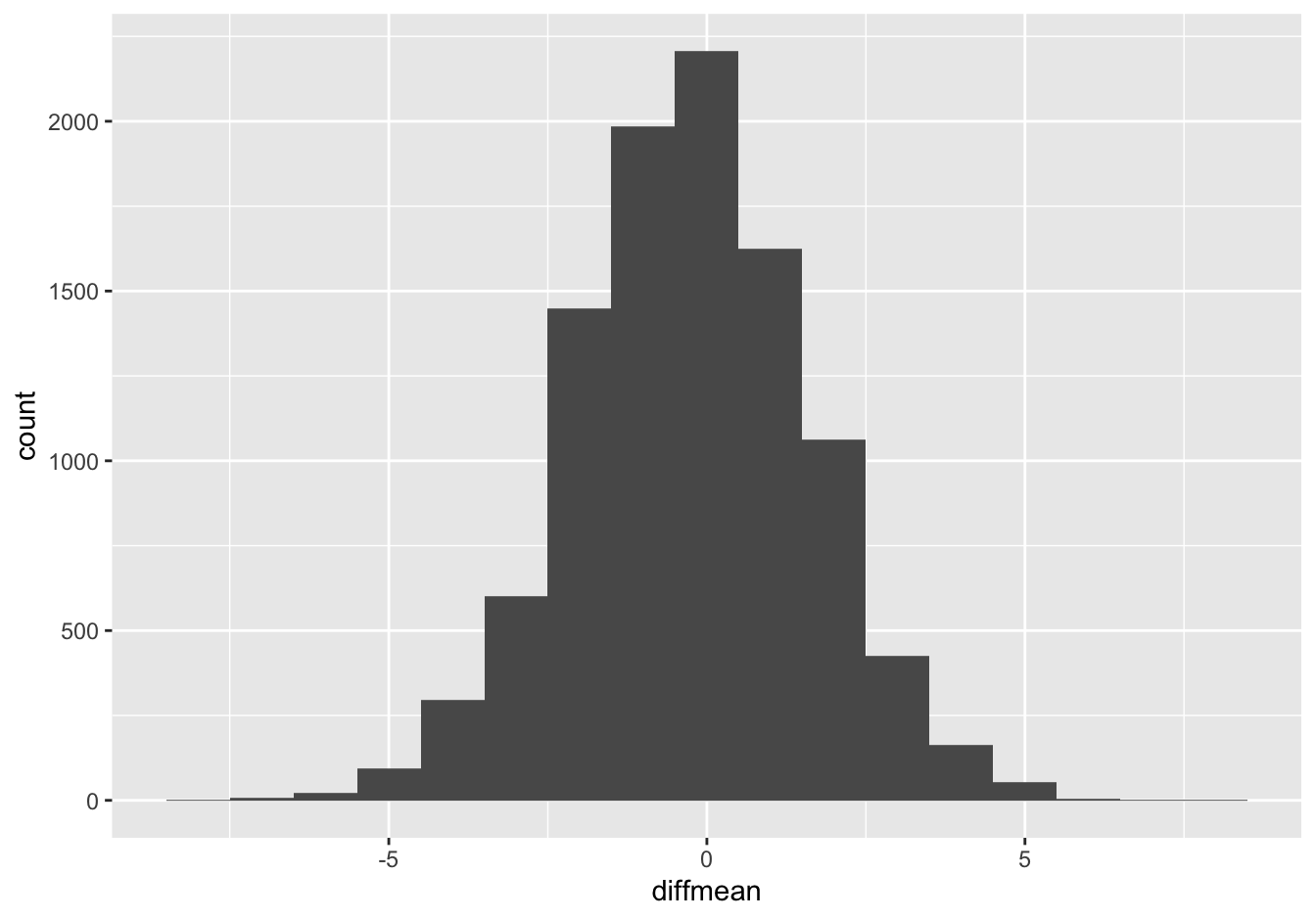

Just eyeballing the histogram, it looks like about 95% of the differences are between -4 hours (female sleeps longer) and +3 hours (male sleeps longer). Compare this distribution with the sampling distribution for the difference of means, above. As is pretty much always the case, the data distribution is much wider than the confidence interval for the mean of that data distribution.

Example 2: smoking and depression

Let’s look at a second example and ask the question: does the frequency of smoking vary according to whether someone reports any days where they feel depressed? Let’s calculate smoking rates stratified by the DepressedAny variable:

prop(Smoke100 ~ DepressedAny, data=NHANES_sleep)

##  prop_No.TRUE prop_No.FALSE 
##     0.4592593     0.5794451

This takes a bit of effort to parse. It’s saying that:

among those with at least one depressed day per month (DepressedAny = TRUE), the proportion of nonsmokers (Smoke100 = "No") is about 46%.
among those with at least no depressed days (DepressedAny = FALSE), the proportion of nonsmokers (Smoke100 = "No") is about 58%.

Altogether, that means that that those reporting at least some symptoms of depression are 12% more likely to have smoked at least 100 cigarettes in their lives:

diffprop(Smoke100 ~ DepressedAny, data=NHANES_sleep)

##  diffprop 
## 0.1201859

Let’s characterize the statistical uncertainty of this number. That is, how precisely can this difference for our sample characterize the corresponding difference in smoking rates for the wider American population? We can use the bootstrap to find out:

boot_smoke_depression = do(10000)*diffprop(Smoke100 ~ DepressedAny, data=mosaic::resample(NHANES_sleep))

This statement says to: 1) create 10,000 bootstrap samples from the original NHANES_sleep data frame, and 2) for each bootstrap sample, recompute the difference in the proportions of the Smoke100 variable respondents with and without at least one depressed day per month. We store the resulting set of 10,000 bootstrapped differences in an object called boot_smoke_depression.

As always, let’s visualize this sampling distribution in a histogram, and then use it to create a confidence interval:

ggplot(boot_smoke_depression) + 
  geom_histogram(aes(x=diffprop))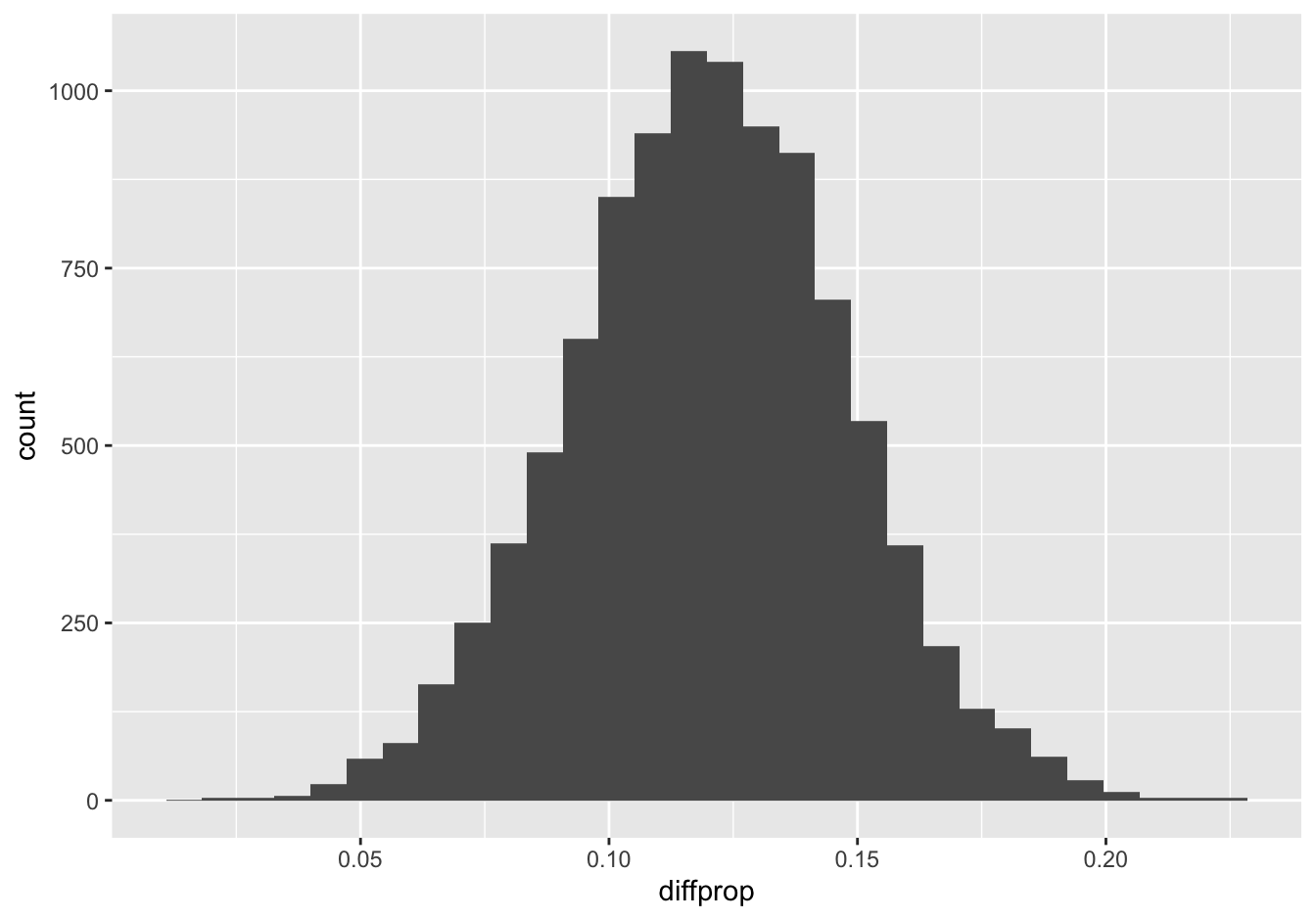

confint(boot_smoke_depression, level = 0.95)

##       name      lower     upper level     method  estimate
## 1 diffprop 0.06634904 0.1731429  0.95 percentile 0.1201859

Based on this survey, it’s clear that those with at least one depressed day per month are more likely to smoke, on average. Our best guess is that there’s a 12% difference in smoking rates, with a 95% confidence interval from 6.6–17.3%. Because this confidence interval doesn’t contain zero, we can say that the difference is statistically significant at the 5% level.

Notice that this result doesn’t say anything about causality. We can’t tell if people are more likely to smoke because they’re depressed, or more likely to become depressed if they’ve smoked, or if both smoking and depression are symptoms of a common cause. In fact probably all three happen in real life, but we can’t even say which is more common on average. All we can say is that there’s a difference in the frequency of depression by smoking status, and how big we think that difference might be for the whole population. The data just give us a fact; it’s up to us how we explain that fact.

9.4 Bootstrapping regression models

Example 1: sleep versus age

Have you ever heard a 30- or 40- or 50-something complain that, with the pressures of work and kids and having to pee in the middle of the night, they sleep less than they used to? No doubt this is true for plenty of individual 30- or 40- or 50-somethings. (As I write this, I am a 30-something with a toddler at home, and it is definitely true for me.) But is it true at the population level? That is, do older people sleep fewer hours than younger people, on average?

Let’s make a quick scatter plot of the data to find out:

ggplot(NHANES_sleep) + 
  geom_jitter(aes(x=Age, y=SleepHrsNight), alpha=0.1)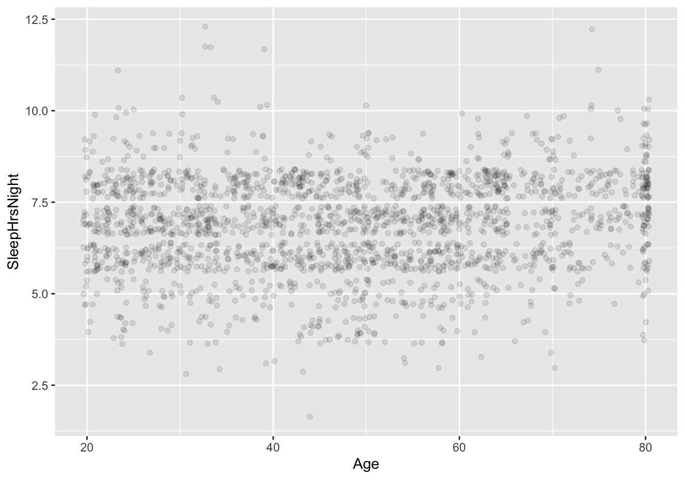

Two quick notes here. First, geom_jitter is just a version of geom_point that injects a tiny bit of artificial jitter, solely for plotting purposes, so that the individual points can be distinguished from one another. (If that doesn’t make sense, try using geom_point instead and you’ll see what I mean.) Second, alpha = 0.1 makes the points only 10% opaque (and 90% translucent).

OK, back to the plot itself. I don’t know about you, but I don’t see any obvious correlation between sleep hours and age from this plot! Already I’m beginning to get suspicious of the idea that age has much to do with sleep.

However, this is where a regression model might help us. Regression models are useful for quantifying relationships in data, even (or perhaps especially) when those relationships might be too subtle to stand out as “obvious” in a plot. So let’s fit a linear model for SleepHrsNight versus age:

lm_sleep_age = lm(SleepHrsNight ~ Age, data=NHANES_sleep)
coef(lm_sleep_age)

## (Intercept)         Age 
##  6.56188885  0.00658811

The coefficient on Age is actually positive: 0.006 extra hours of nightly sleep with each additional year of age, or equivalently, about 3.6 minutes extra nightly sleep with each passing decade. This is certainly not consistent with the idea that older people sleep fewer hours than younger people, on average. (As an aside, it also provides another example of a non-interpretable intercept: construed literally, this intercept would imply that newborns sleep 6.6 hours per night, which I assure you is not true. It’s just an artifact of extrapolating our model’s predictions way beyond where we have data.)

Moreover, now that we know how to bootstrap, we can also measure the statistical uncertainty of our slope estimate, like this:

boot_sleep_age = do(10000)*lm(SleepHrsNight ~ Age, data=mosaic::resample(NHANES_sleep))

This statement says to: 1) create 10,000 bootstrap samples from the original NHANES_sleep data frame, and 2) for each bootstrap sample, refit a linear model (lm) for SleepHrsNight versus Age. We store the resulting set of 10,000 fitted regression models in an object called boot_sleep_age.

Now we can ask for a confidence interval based on this bootstrapped sampling distribution:

confint(boot_sleep_age, level = 0.95)

##        name       lower        upper level     method    estimate
## 1 Intercept 6.391943250  6.733946180  0.95 percentile 6.687634681
## 2       Age 0.003300173  0.009896674  0.95 percentile 0.005504169
## 3     sigma 1.266747848  1.359503814  0.95 percentile 1.359390771
## 4 r.squared 0.001838715  0.016681751  0.95 percentile 0.004924458
## 5         F 3.663940492 33.742893754  0.95 percentile 9.843218969

There’s a lot of information in this table that we haven’t yet learned to interpret. But for now, focus only on the Age row. This row is telling us the lower and upper bounds for our 95% confidence interval on the Age coefficient in our linear model. To be specific, we’re 95% confident that the true population-wide slope of sleeping hours versus age is somewhere between 0.003 and 0.010 extra hours per night, each additional year of age—or equivalently, between 1.8 and 6 extra minutes of sleep per night per decade.

To provide some context for this confidence interval, it helps to see the fitted line superimposed on top of the data, like this:

ggplot(NHANES_sleep) + 
  geom_jitter(aes(x=Age, y=SleepHrsNight), alpha=0.1) + 
  geom_smooth(aes(x=Age, y=SleepHrsNight), method='lm')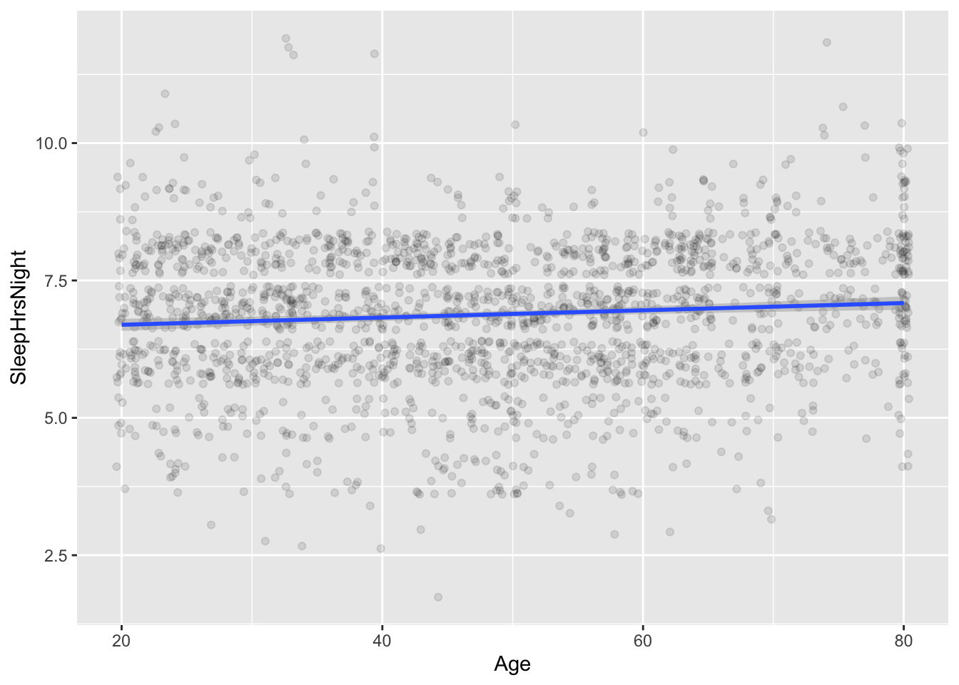

The line is essentially, but not exactly, flat.

Statistical vs. practical significance

This example serves to illustrate a really important distinction in data science: the distinction between statistical significance and practical significance.

As we’ve already discussed, statistical significance just means whether the confidence interval for some estimate contains zero—nothing more, nothing less. By this narrow definition, the relationship between age and sleeping hours per night is statistically significant at the 5% level. After all, the 95% confidence interval for the Age slope doesn’t contain zero:

confint(boot_sleep_age, level = 0.95) %>% filter(name == 'Age')

##   name       lower       upper level     method    estimate
## 1  Age 0.003300173 0.009896674  0.95 percentile 0.007623065

Practical significance, on the other hand, means whether the numerical magnitude of something is large enough to matter to actual human persons, as opposed to statisticians performing their day jobs. This is necessarily a subjective judgment: “large enough to matter” is not a well-defined mathematical term. But it’s often pretty obvious in context. After all, ask yourself: in subjective terms, does 3.6 minutes of extra nightly sleep with each decade sound like a lot to you? It certainly doesn’t to me. And in more objective terms, 3.6 minutes also doesn’t seem large in the context of the intrinsic variability in SleepHrsNight across the population, with a standard deviation of…

sd(~SleepHrsNight, data=NHANES_sleep)

## [1] 1.317419

…1.3 hours, or 78 minutes per night.

So yes, there is a “statistically significant” relationship between age and sleep hours. This relationship is, contrary to the short-term experience of new parents, actually positive. On average, older adults sleep a bit more than younger adults.³²

But only on average, and even then only a little bit! Don’t fall into the trap of assuming that, just because some effect is labeled “statistically significant,” it must therefore matter in the real world. It just isn’t so. The age–sleep relationship in the NHANES data is a perfect example of an effect that is statistically significant, but that we’re nearly sure, based on the confidence interval, must be so small that it hardly matters at all in practical terms. (Again, that’s my opinion; if 3.6 minutes of extra sleep is make-or-break for you, you’re certainly free to disagree, but sadly the data suggest that you’ll need to wait a decade for those coming nights of somnolent bliss.)

Now, don’t get me wrong. I’m not saying that statistical significance is an irrelevant concept. Being able to speak the language of statistical significance is really important for communicating about data. Rightly or wrongly, there are times and places where people just expect you to use the term, especially in certain allegedly rarefied academic contexts. More to the point, there are also cases, like in clinical trials, where it actually is super important to know whether an effect is statistically significant. (Does this new drug actually work better than the old one? Does this new vaccine work at all?)

But confidence intervals are almost always more useful than claims about statistical significance. My advice to you is to entertain the full range of values encompassed by the confidence interval, rather than jumping straight to the needlessly binary question of whether that confidence interval contains zero.

In fact, I’ll tell you a little secret. Sometimes people use the term “statistical significance” to sound fancy and scientific and credible. Sometimes it even works. But to those who know better, focusing too much on statistical significance, at the expense of focusing on practical significance, instead comes across as a mark of insecurity or pseudo-seriousness about statistics.

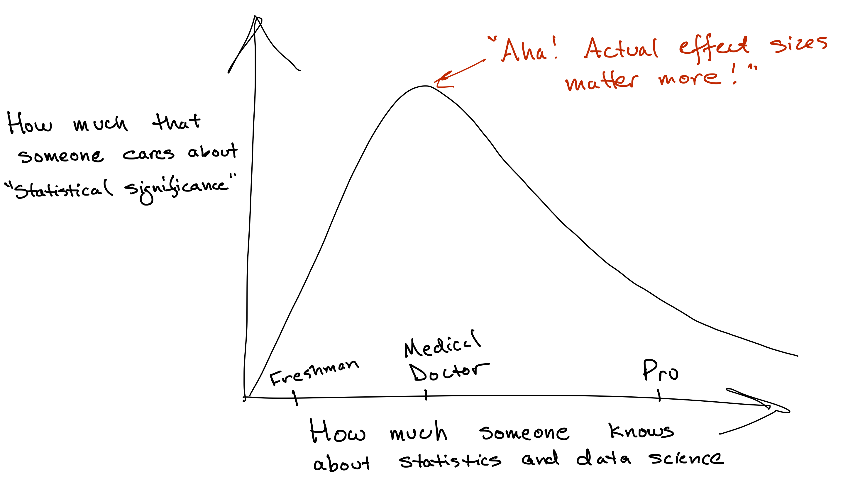
That’s because there are at least three more important questions than whether an effect is statistically significant.

How big is the effect, in practical terms?
How much statistical uncertainty is there surrounding that effect?
Is statistical uncertainty even the dominant contribution to real-world uncertainty about the effect? (See “The truth about statistical uncertainty.”) Or might there be a large hidden bias in the measurement process, potentially turning any discussion of statistical uncertainty into a pointless academic exercise?

Once you get in the habit of asking these questions, the significance question—“Could the effect be exactly zero, up to statistical uncertainty?”—can start to feel a bit silly.

Moreover, there’s also an unfortunate glory-hound phenomenon related to this whole discussion about statistical significance. Consider two newspaper headlines you could write based on our analysis of the NHANES data:

Age a significant predictor of sleep patterns, new study finds

Age nearly irrelevant in explaining sleep patterns, new study finds

Paradoxically, both headlines are true. But the first one is true only in a narrow pedantic sense. It pulls a fundamentally dishonest trick; it expects that you’ll read “significant” as meaning “having a large effect in the real world,” rather than as “statistically significant at the 5% level.” Note that this probably isn’t a trick played by the journalist on the reader. It’s more likely to be a trick played by the study authors on both themselves and the journalist, because none of them know any better.

I hope you agree that the first headline is basically fake news. But while the second headline may be non-fake, it is also, sadly, non-news—both to sleep researchers and to the general public. Very few headlines of the form “Study finds no big deal” have ever been written, either in newspapers or academic journals. You can therefore imagine which headline a journalist would rather write, and which study an academic would rather try to publish—maybe out of ignorance, maybe out of “publish or perish” career insecurity, but definitely to the detriment of public knowledge and trust in science.

This emphatically doesn’t mean that all academic studies are just dumb stats tricks published by glory hounds. (See: mRNA vaccines.) But it does mean that it’s hard to tell from a newspaper headline whether any specific academic study is just a dumb stats trick published by glory hounds. There’s only one antidote. Read the study. Look for the confidence interval. Judge for yourself!

Example 2: West Campus rents

Let’s see a second example of bootstrap confidence intervals for a regression model. Here, we’ll try to answer a question about the Austin real-estate market that’s very much on the minds of many UT-Austin students: how do apartment rents in the West Campus neighborhood fall off as you get further away from campus itself?

Please download and import the data in apartments.csv, which contains data on a sample of 67 apartments in West Campus. For each apartment, we know the monthly rent and square footage of a two-bedroom apartment, as well as the distance from the UT Tower, which marks the notional (if not the actual) center of campus. (The data set has several other feature of the unit that might affect price, but we’re not concerned about those here.) This analysis focuses on two-bedroom apartments, since virtually all buildings have many units of this size, and since we want a common basis for comparing across buildings.

Here are the first several lines of the file. The relevant variables for our purposes are two_bed_rent, measured in dollars per month, and distance_from_tower, measured in miles:

head(apartments)

##          residence twobed_rent twobed_sf furnished pool distance_from_tower laundry_in_unit electricity water
## 1         21 Pearl        1010       777     FALSE    0                 0.6               1           0     0
## 2           21 Rio        1149       975     FALSE    1                 0.5               1           0     0
## 3      2400 Nueces        1250       802      TRUE    1                 0.3               1           1     1
## 4          26 West        1084      1014      TRUE    1                 0.5               1           0     0
## 5         900 West         900       837     FALSE    0                 0.7               0           0     0
## 6 Axis West Campus        1189      1024      TRUE    1                 0.6               1           0     0
##                                 address y_coordinate x_coordinate utilities
## 1 Pearl St & W 21st St Austin, TX 78705     30.28414    -97.74662        no
## 2   2101 Rio Grande St Austin, TX 78705     30.28430    -97.74473        no
## 3       2400 Nueces St Austin, TX 78705     30.28838    -97.74343       yes
## 4        600 W 26th St Austin, TX 78705     30.29075    -97.74349        no
## 5          900 W. 23rd Austin, TX 78705     30.28750    -97.74690        no
## 6     2505 Longview St Austin, TX 78705     30.29016    -97.75046        no

Let’s build a linear regression model for rent versus distance from the UT Tower:

lm_distance = lm(twobed_rent ~ distance_from_tower, data=apartments)
coef(lm_distance)

##         (Intercept) distance_from_tower 
##           1366.8075           -631.5061

This suggests a drop-off in rent of about $631 per mile from the Tower, on average. That’s a pretty steep price gradient, but it reflects the limited supply of (and intense demand for) properties close to campus.

What about a confidence interval for that slope? Let’s bootstrap:

boot_distance = do(10000)*lm(twobed_rent ~ distance_from_tower, data=mosaic::resample(apartments))
confint(boot_distance, level = 0.95)

##                  name         lower        upper level     method     estimate
## 1           Intercept 1226.69639101 1509.8281264  0.95 percentile 1370.5576796
## 2 distance_from_tower -841.04718571 -415.6242279  0.95 percentile -642.5329598
## 3               sigma  112.85095881  214.6316079  0.95 percentile  164.9187693
## 4           r.squared    0.08598215    0.4501045  0.95 percentile    0.2408417
## 5                   F    6.11458475   53.2042767  0.95 percentile   20.6211404

So our 95% confidence interval ranges from about -$840 per mile to about -$420 per mile. (The numbers are negative because increased distance implies lower price, on average. Also, I feel OK rounding to the tens place because the confidence interval says the number isn’t certain even to the hundreds place; further precision beyond the tens place is pointless).

This is an example of a relationship that is both statistically significant (because the confidence interval doesn’t contain zero) and practically significant (because all the values in the confidence interval look large, in real-world terms). To reason a bit more specifically about practical significance, lets assume 1 mile equals a 20-minute walk, and therefore 0.1 miles equals a 2-minute walk. So to save 2 minutes each way in walking distance, you’d expect to pay an extra 0.1 $\times$ 630 = $63 per month for a two-bedroom West Campus apartment. Or maybe, if this is an especially unlucky sample, you’d expect to pay 0.1 $\times$ $420 = $42 on average, across all apartments in the general population—but that’s only on the very low end of the confidence interval. No matter what, it seems like a big effect.

9.5 Bootstrapping usually, but not always, works

Let’s turn now to a question that may have occurred to you already: how do I know this bootstrap thing actually works? Take the specific example of this bootstrap confidence interval we calculated earlier, for the average number of hours per night that Americans sleep:

boot_sleep = do(10000)*mean(~SleepHrsNight, data=mosaic::resample(NHANES_sleep))
confint(boot_sleep, level = 0.95)

##   name    lower    upper level     method estimate
## 1 mean 6.820191 6.937217  0.95 percentile 6.878955

When I calculate this interval and state, “I’m 95% confident that the average sleep time in America is between 6.82 and 6.94 hours per night,” what reason do you have to believe me? I’m sure you are a streetwise, highly experienced individual. Indeed, I’ve heard tell of your legend. Your sniffer is sound. Your compass is true. On many occasions, you’ve heard someone make statements with a high degree of self-professed confidence, while you’ve known the whole time that they were totally full of shit. What, if anything, makes my statement, and my self-professed confidence, any different?

What “confidence” means

I’d argue that one very good reason to have confidence in someone is because they have a track record of making truthful statements. It’s why people generally trust nurses and school teachers, but not politicians or men on dating apps.

This very same notion of confidence is fundamental to data science. It helps to start with an analogy. Imagine, for example, the following conversation between two quality-control engineers on an assembly line for smart phones.

Alice: Hi Bob!

Bob: Hi, Alice! Listen, you know that last phone that just came off the assembly line? Is it actually working correctly? We should probably check.

Alice: I’m 99.9% confident that it’s working correctly.

Bob: Wait, what? 99.9%? Why don’t you just turn it on and check? Then you’ll know for sure.

Alice: Do you even work here? This phone doesn’t have a battery in it yet. Who do I look like, the Evil Emperor from Star Wars? I can’t just shoot electricity out of my fingers and turn it on.

Bob: So how are you 99.9% confident that it’s working?

Alice: Well, we make 10,000 phones a day here, and on average, only about 10 of them fail our quality-control checks later in the process, after their batteries are installed. That’s a 99.9% track record. I’m therefore 99.9% confident that this particular phone is working just fine.

Bob: OK, that makes sense!

When it comes to data science, we can formalize this idea of a track record in terms of something called the “coverage principle.”

Definition 9.2 The coverage principle: if you were to analyze one data set after another for the rest of your life, and you were to construct X% confidence intervals for every estimate you made, those intervals should cover (i.e. contain) their corresponding true values at least X% of the time. Here X can be any number between 0 and 100.

With that definition in place, let’s now imagine a second conversation, this one between two sleep researchers.

Bob: Hey, Alice, you know that sleep study you were working on yesterday? What did you learn from the results?

Alice: I’m 95% confident that Americans sleep between 6.82 and 6.94 hours per night, on average.

Bob: Wait, what? 95%? Why don’t you just ask people and check? Then you’ll know for sure.

Alice: Do you even work here? That would entail surveying more than 300 million people, or maybe tricking them all into downloading spyware that listens for snoring. Who do I look like, the Evil Emperor from Facebook? I don’t have that kind of time, budget, or filth in my soul.

Bob: So how are you 95% confident in your answer?

Alice: Well, I’ve made 10,000 confidence intervals in my life using this exact same data-analysis procedure, and only about 500 of them ended up failing to contain the true value I was aiming at, after other researchers looked into it and the right answer became more or less known. That’s a 95% track record. I’m therefore 95% confident that this particular interval contains the right answer.

Bob: OK, that makes sense!

There is an appealing simplicity here: if you’re going to claim 95% confidence, you should be right at least 95% of the time over the long run. You’ll notice that, in both cases, Alice’s stated level of confidence was ultimately a claim about the track record of some specific procedure—a procedure for building smart phones in one case, and a procedure for building confidence intervals in the other.

Well, we’ve learned only one procedure for building confidence intervals, and that’s the bootstrap. The key question, then, is actually pretty simple. Does the bootstrap have a good track record? More specifically, does bootstrapping, as a procedure for building confidence intervals, actually satisfy the coverage principle, as laid out in Definition 9.2?

The answer is: basically, yes! A slightly more nuanced answer is: usually and approximately. We’ll first see an example where the bootstrap does indeed work very well, which is actually pretty representative of most common data-science situations. After that we’ll see a trickier case where the bootstrap doesn’t work well at all.

Example 1: sample mean

Please once again import the rapidcity.csv data set from a previous lesson, containing daily average temperatures (the Temp column) in Rapid City, SD over many years.

You might remember that the average temperature in Rapid City over this entire time period (1995-2011) was about 47.3 degrees F:

mean(~Temp, data=rapidcity)

## [1] 47.28159

There’s no statistical uncertainty associated with this number. We can think of it as a “population” mean, because our data set is effectively a census: it contains every day from the beginning of 1995 to the end of 2011. (There would be uncertainty if we wanted to use this number make a guess about the average temperature over other time periods, but that’s not our goal here.)

But instead of working from this census, now imagine that we took a sample of, say, 50 days, and tried to estimate the population average of 47.28 degrees. Although this seems kind of artificial here, where we actually do have the census, it’s a good working model for how sampling works in the real world, and therefore a good way to assess whether the bootstrap performs well as a procedure for building confidence intervals based on samples.

Here’s our sample of size 50, along with the corresponding sample mean.

rapidcity_sample = sample_n(rapidcity, 50)
mean(~Temp, data=rapidcity_sample)

## [1] 49.382

Of course we don’t get the right answer, which is 47.28. But what if we now bootstrap that sample to construct a confidence interval? Notice that, crucially, our code below resamples from the “temperature sample” in the rapidcity_sample data set we just created above, but not the full “temperature census” in rapidcity:

rapidcity_sample_boot = do(1000)*mean(~Temp, data=mosaic::resample(rapidcity_sample))
confint(rapidcity_sample_boot, level = 0.95)

##   name   lower   upper level     method estimate
## 1 mean 43.4932 54.7334  0.95 percentile   49.556

It looks like our bootstrap confidence interval contains the right answer of 47.28. That’s a good result.

Did we just get lucky? Let’s try it again. First we’ll take an entirely new sample of size 50, and use that new sample to once again estimate the population average:

rapidcity_sample2 = sample_n(rapidcity, 50)
mean(~Temp, data=rapidcity_sample2)

## [1] 47.264

Once again, we don’t get the right answer, which is 47.28. But let’s bootstrap this second sample to get a confidence interval:

rapidcity_sample_boot2 = do(1000)*mean(~Temp, data=mosaic::resample(rapidcity_sample2))
confint(rapidcity_sample_boot2, level = 0.95)

##   name   lower    upper level     method estimate
## 1 mean 40.6504 53.77645  0.95 percentile   44.708

And again, our bootstrap confidence interval contains the right answer of 47.28. We’re 2 for 2. Do you trust the bootstrap yet?

If not, perhaps 100 confidence intervals from 100 different samples will persuade you? Let’s try it. My code block below uses some more advanced R tricks to run this simulation, so don’t worry too much about the details. I don’t expect you to understand or replicate each line of this code; I include it merely so you can see how I get the result you’ll see below. (The code is made a bit harder to read because it takes advantage of the fact that my machine has 8 compute cores on it, which allows me to parallelize the computational heavy lifting here.)

library(foreach)
library(doParallel)
registerDoParallel(8)

one_hundred_intervals = foreach(iter = 1:100, .combine='rbind') %dopar% {
  rapidcity_sample = sample_n(rapidcity, 50)
  rapidcity_sample_boot = do(1000)*mean(~Temp, data=mosaic::resample(rapidcity_sample))
  confint(rapidcity_sample_boot, level = 0.95) %>%
    mutate(Sample = iter)
}

one_hundred_intervals = one_hundred_intervals %>%
  mutate(contains_truth = ifelse(lower <= 47.28 & upper >= 47.28,
                                 yes="yes", no = "no"))

This code draws 100 real samples of size 50 from the original data set. Then for each of those real samples, we:

Draw 1000 bootstrap samples, and for each one compute the bootstrap sample mean.
From that bootstrap sampling distribution of 1000 means, compute a confidence interval.
Check whether the confidence interval contains the right answer of 47.28.

The code takes 10 or 15 seconds to run even with 8 compute cores, but the result is 100 samples leading to 100 confidence intervals, about 95 of which should contain the truth. To check, let’s make a plot using geom_errorbar, which we haven’t specifically learned about yet, but which is tailor-made for showing confidence intervals:

ggplot(one_hundred_intervals) + 
  geom_errorbar(aes(x=Sample, ymin=lower, ymax=upper, color=contains_truth)) + 
  geom_hline(aes(yintercept = 47.28), color='black') + 
  theme(legend.position="bottom")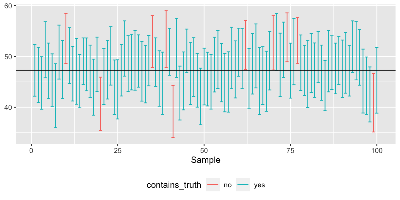

Figure 9.3: The best self-diagnostic I know for assessing your understanding of the bootstrap.

Bingo! Each of the vertical bars represents a single confidence interval from a single sample. The true value is shown as a horizontal line at 47.28 degrees; you’ll recall this number was based on our “temperature census,” i.e. the full 1995–2011 data set from which we drew the samples. The blue intervals contain that true value. The red intervals don’t. I count 7 red intervals out of 100, or equivalently, 93 blue intervals out of 100. That’s pretty close to 95%.

Incidentally, I’ve found over the years that Figure 9.3, with its 100 different confidence intervals, is an excellent self-diagnostic. If you understand this figure—I mean really understand it, like how it was constructed, why it was constructed that way, and what it actually implies—then congratulations! You should be proud of yourself, because to understand this figure, you have to understand a whole heck of a lot:

what we’re measuring when we measure “statistical uncertainty.”
what a sampling distribution is and why it’s important.
what bootstrapping is and how it works.
how to get a confidence interval from a bootstrap sampling distribution.
what basis we might have for trusting a data scientist when they say “I’m 95% confident.”
why bootstrapping seems, at least on the initial evidence, worthy of that trust.

In other words, if you understand this figure, you’ve basically aced the last two lessons.³³ On the other hand, if you don’t understand it, you have a deficit somewhere in need of a remedy. I suggest revisiting the last two lessons, proceeding only when you feel comfortable with each of the bullet points above.

Example 2: sample minimum

Just so that you don’t come away from this lesson thinking that the bootstrap always works, let’s see a case where it doesn’t.

What was the lowest daily average temperature in Rapid City between 1995 and 2011? Answer:

min(~Temp, data=rapidcity)

## [1] -19

-19 degrees F, or -28 C. Let’s call this our “population minimum,” at least for the period 1995–2011. As with the “population mean” of 47.28 F, there’s no statistical uncertainty associated with this number.

But now let’s take a sample of 50 days, just as we did before, and try to use the minimum of that sample to estimate this population minimum. Here’s one sample of size 50, along with the corresponding minimum temperature in that sample:

rapidcity_sample = sample_n(rapidcity, 50)
min(~Temp, data=rapidcity_sample)

## [1] 18.8

Well, that’s not very close. Then again, of course our sample answer is wrong, compared with the right answer of -19. We should expect to see that by now for pretty much any statistical summary. So let’s bootstrap our sample and calculate a confidence interval:

rapidcity_sample_boot_min = do(1000)*min(~Temp, data=mosaic::resample(rapidcity_sample))
confint(rapidcity_sample_boot_min, level = 0.95)

##   name lower upper level     method estimate
## 1  min  18.8  25.2  0.95 percentile     18.8

It looks like our bootstrap confidence interval ranges from 18.8 to 25.2. Wow. That’s a horrible miss, considering the right answer for the “population” minimum is -19.

Did we just get unlucky? After all, a 95% confidence interval should miss 5% of the time. Maybe we just experienced that 5%.

So let’s try it again. First we’ll take an entirely new sample of size 50, and use the minimum of that new sample to again estimate the population minimum:

rapidcity_sample2 = sample_n(rapidcity, 50)
min(~Temp, data=rapidcity_sample2)

## [1] 11

Once again, we don’t get the right answer of -19—but that’s expected. So let’s bootstrap this second sample to get a confidence interval:

rapidcity_sample_boot_min2 = do(1000)*min(~Temp, data=mosaic::resample(rapidcity_sample2))
confint(rapidcity_sample_boot_min2, level = 0.95)

##   name lower upper level     method estimate
## 1  min    11  22.3  0.95 percentile       11

Missed again! We’re 0 for 2. What’s going on?

Let’s more carefully verify that this isn’t just bad luck, by repeating our exercise of simulating 100 separate samples and calculating a bootstrap confidence interval for each one. Except instead of bootstrapping the sample mean, we’ll bootstrap the sample minimum.

Here’s my modified code block to do just that. I basically just copied and pasted from above, changing mean to min:

registerDoParallel(8)
another_one_hundred_intervals = foreach(iter = 1:100, .combine='rbind') %dopar% {
  rapidcity_sample = sample_n(rapidcity, 50)
  rapidcity_sample_boot = do(1000)*min(~Temp, data=mosaic::resample(rapidcity_sample))
  confint(rapidcity_sample_boot, level = 0.95) %>% 
    mutate(Sample = iter)
}

another_one_hundred_intervals = another_one_hundred_intervals %>%
  mutate(contains_truth = ifelse(lower <= -19 & upper >= -19,
                                 yes="yes", no = "no"))

Let’s now plot these 100 confidence intervals and check how many of them contained the true population minimum.

ggplot(another_one_hundred_intervals) + 
  geom_errorbar(aes(x=Sample, ymin=lower, ymax=upper, color=contains_truth)) + 
  geom_hline(aes(yintercept = -19), color='black') +
  theme(legend.position="bottom")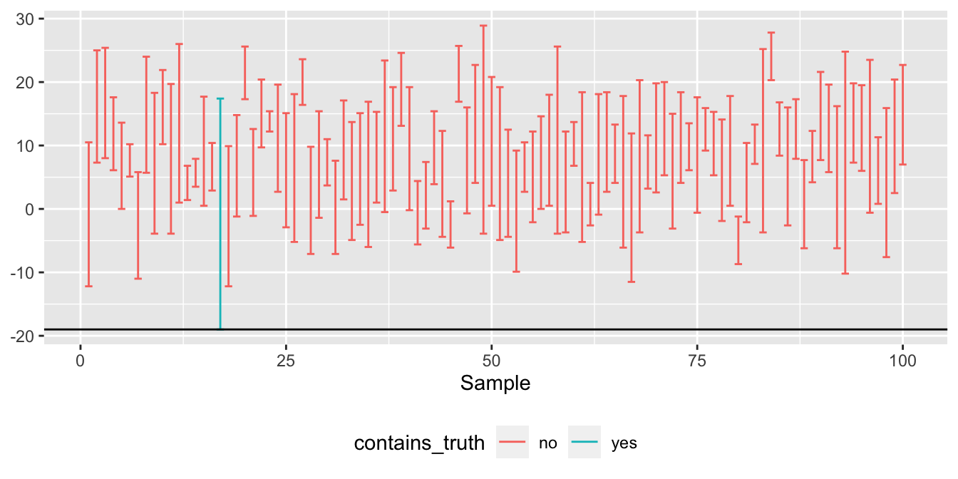

Figure 9.4: This is about as bad as bootstrapping gets.

Holy cow. Of our 100 different 95% bootstrap confidence intervals, just one of them actually contained the true value of -19 F. That’s not just bad luck. Something has gone horribly wrong. But what?

What’s wrong is that the lowest temperature in a sample of 50 days is a really naive estimate for the lowest temperature we expect to see over a 16-year (or 5,844 day) period. The only way your sample minimum can ever equal the population minimum is if, by sheer dumb luck, you just happen to sample the very coldest day overall. With a sample size of 50, and a population size of 5,844, the chances that this happens are about 1 in 117. For the other 116 out of 117 samples, the sample minimum is necessarily larger than the population minimum. No matter how many times you bootstrap such a sample, you are never going to hit -19 F, and your confidence interval will fail to contain the true population minimum. So as an estimator of the population minimum, the sample minimum exhibits a massive, fundamental asymmetry: it’s never too low, it’s nearly always too high, and very rarely it’s exactly right. This asymmetric behavior is quite different from that of the sample mean: half the time the sample mean is too low and half the time it’s too high, so that on average it’s about right.

The moral of the story is: the bootstrap doesn’t always work. In particular, it doesn’t work for the min (or max) of a sample!

Closing advice

So we’ve seen one example where the bootstrap works great, and another example where it works horribly. Where does that leave us?

In turns out that our second example, where we tried to bootstrap the sample minimum to get a confidence interval for the population minimum, is a bit pathological. That is to say: it’s not representative of most common data-science situations.

In fact, you can successfully bootstrap most common summary statistics most of the time, assuming your observations can plausibly be interpreted as independent samples from some larger reference population. By “safely,” I mean that you can quote bootstrap confidence intervals in the knowledge that you’re likely to cover the true value the stated percentage of the time. These “safe” statistics include almost all the stuff we’ve been calculating in these lessons so far:

means and medians
standard deviations and inter-quartile ranges
correlations
quantiles of a distribution that aren’t too extreme (e.g. the 25th percentile is OK, but the 99th percentile might not work well unless your sample size is huge)
regression coefficients from ordinary least squares (i.e. from lm in R)
group-wise differences of any of these statistics

I recognize that the phrase “most common summary statistics most of the time” contains not just one but two weasel words in it. That’s because it’s hard to give generic, non-weasely advice about the bootstrap, and about statistical inference more generally, without the discussion veering off into some very deep, very scratchy mathematical weeds. All I’ll say about the math is that our best people are working on it.

However, I can give you some other examples of where the bootstrap breaks, and where you therefore need more advanced inference techniques not covered in these lessons. These include the following situations:

your sample is very small, say less than 20 or maybe 30.
you want to estimate the extreme quantiles of a distribution (of which the min and max are the most extreme possible, as you’ve seen).
your data points are highly correlated across space or time.
you’re fitting a very fancy machine-learning model, with a cool name like “lasso” or “deep neural network.”
the underlying population distribution is very heavy-tailed.

Honestly, this is the kind of stuff you’d learn about in a more advanced statistics course. Your best bet in these cases is to actually take such a course, or else to work with a professional statistician. Of course, if you’d like to dig in more yourself, the following book has a chapter (Ch.9) devoted to “When Bootstrapping Fails Along with Remedies for Failures”:

M. R. Chernick, Bootstrap methods: A guide for practitioners and researchers, 2nd ed. Hoboken N.J.: Wiley-Interscience, 2008.

Study questions: the bootstrap

Return to the NHANES_sleep data. Use bootstrapping the answer the following questions.

How does average sleep time differ for those with and without at least one depresssed day per month? Calculate a 95% confidence interval for the difference in the mean of SleepHrsNight between the two groups. Is the difference statistically significant at the 5% level? In your opinion, is the difference practically significant?
How does the frequency of depression differ by gender? Calculate a 95% confidence interval for the difference in the proportion of DepressedAny = TRUE between the two groups. Is the difference statistically significant at the 5% level? In your opinion, is the difference practically significant?

Let’s ignore the obvious fact that, if you had access to all those parallel universes, you’d also have more data. The presence of sample-to-sample variability is the important thing to focus on here.↩︎
The term “bootstrapping” is a metaphor, from an old-fashioned phrase that means performing a complex task starting from very limited resources. Imagine trying to climb over a tall fence. If you don’t have a ladder, just “pull yourself up by your own bootstraps.”↩︎
This isn’t a theorem or anything; it’s just something I’ve noticed because I use the bootstrap a lot, and I therefore end up comparing it to more “bespoke” options in a bunch of different situations. For the kinds of problems that we tend to look at in an intro data science course, it’s a rare case that I notice much of a practical difference between the answer I get from the bootstrap and the answer I get from some other, more clever, more situation-specific technique for inference.↩︎
There are varieties of the bootstrap designed for other forms of randomness, including the parametric bootstrap and the residual resampling bootstrap. There’s also a technique called the randomization test or permutation test that has a very bootstrap-like feel, and is explicitly designed to measure statistical uncertainty association with experimental randomization.↩︎
We can often get away without adding the mosaic::, but it’s better to be sure that R knows which version of resample we want. In particular, if you load tidyverse first and mosaic second, R should assume automatically that you want the version of resample from mosaic and not from any of the tidyverse packages.↩︎
This is a tad misleading. A more detailed look at the NHANES data shows a small average dip in average sleep time from from ages 20-50, and then a small rise from ages 50-80. But the rise at the back end is a bit steeper than the dip at the front end, for a small net-positive average effect from ages 20-80.↩︎
To be clear, it’s not important that you understand the micro-level details of the R code block I provided. Nor is it important that you could actually code this kind of thing yourself. What is important is that you understand the high-level tasks that my code block is accomplishing.↩︎