Lesson 5 Summaries
In this lesson, you’ll learn to calculate basic summary statistics for numerical variables, including:
- means and medians to measure the typical value in a data set.
- standard deviations and IQRs to measure variation from the typical value.
- min, max, and, and quantiles to measure the extremes.
- \(z\)-scores, to make standardized comparisons of fundamentally different types of quantities.
This lesson is all about numerical variables. It’s therefore analogous to our lesson on Counting, which focused on summarizing categorical variables by making tables of counts and proportions. Between this lesson and that one, you’ll have covered the most common data summaries for the two basic types of variables (numerical and categorical).
To get started, create a fresh new script, and then load the tidyverse library by placing the following line at the top of your script and running it in the console:
library(tidyverse)Please also import the rapidcity.csv data set, which you saw in the previous lesson, and which contains daily average temperatures in Fahrenheit (the Temp column) in Rapid City, SD over many years. My code below assumes that you’ve imported the data set into an object called rapidcity, which will be the default object name if you used the Import Dataset button. If you need a refresher on importing data, see here.
The Temp column, measured in degrees F, shows the average daily temperature, which is the midpoint between that day’s high and low temps. Let’s begin by re-examining the histogram of daily temperatures that we saw in a prior lesson.
ggplot(rapidcity) +
  geom_histogram(aes(x=Temp), binwidth=2)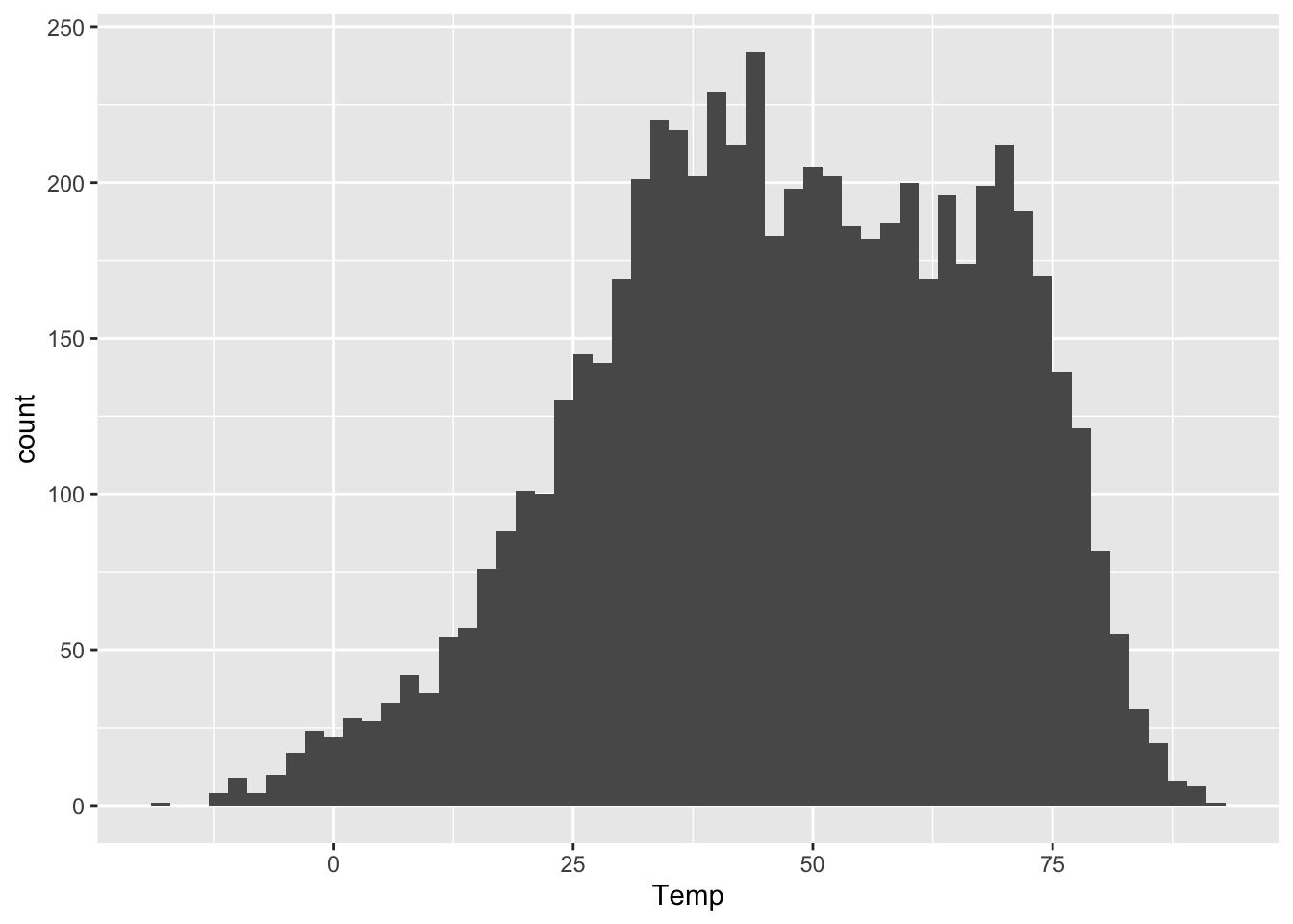
Statistical summaries entail distilling a complex data distribution like this one into a few simple numbers that answer questions like these.
- the typical value: what’s the temperature on a typical day in Rapid City? (
meanandmedian)
- the variation: how much do the individual days vary from a “typical” day? (
sdandIQR) - the extremes: what temperatures should we expect on days that are unusually hot or unusually cold (at least, for Rapid City)? (
min,max, andquantile)
We’ll step through the Rapid City temperature data one summary at a time, building up a list of statistics bit by bit.
5.1 The typical value
Two conventional ways to measure the typical value in a data set are the mean and the median.
There are many ways we can calculate a mean in R. The way I’m going to show isn’t actually the most concise, at least for a simple summary like the mean. But it is very transparent, and it also has the virtue of generalizing much more readily to situations where we want to calculate more complex summaries.
Here’s my preferred way in R to calculate a mean. This uses pipes (%>%); if you need a refresher on pipes, revisit this lesson.
rapidcity %>%
  summarize(avg_temp = mean(Temp))
## avg_temp
## 1 47.28159So about 47.3 degrees F. Let’s look at this statement piece by piece:
- we start by piping (
%>%) therapidcitydata set into thesummarizefunction, which—as its name suggests—is the function in R for computing data summaries.
- inside the parentheses of the
summarizefunction, we have an assignment statement,avg_temp = mean(Temp)…- The right-hand side of this statement,
mean(Temp), tells R what summary statistic to calculate. Here we calculate the mean of theTempvariable.
- The left-hand side of the statement,
avg_temp, is what name we want to give this summary.
- The right-hand side of this statement,
We can calculate the median, or the middle value in a sample, in a very similar way. Let’s augment our summary pipeline to calculate both the mean and median, so we can compare them:
rapidcity %>%
  summarize(avg_temp = mean(Temp),
            median_temp = median(Temp))
## avg_temp median_temp
## 1 47.28159 47.6As you can see from this example, the summarize function lets you calculate as many summaries as you want, separated by commas. You don’t have to put each summary on a separate line the way I have, nor do you need to indent them so that they all line up. But I find that doing so makes for more readable code.16 Here the mean and median are pretty similar. This will generally be the case when data distribution isn’t too skewed, i.e. unbalanced to the left or right.
On the other hand, for distributions that are highly skewed one way or another, or that contain large outliers, the mean and median can be quite different. In those situations, the median is generally considered a more representative measure of what’s “typical,” because it is less affected by heavy tails and outliers.
Consider, for example, the distribution of U.S. household income in 2010, which is heavily skewed to the right:
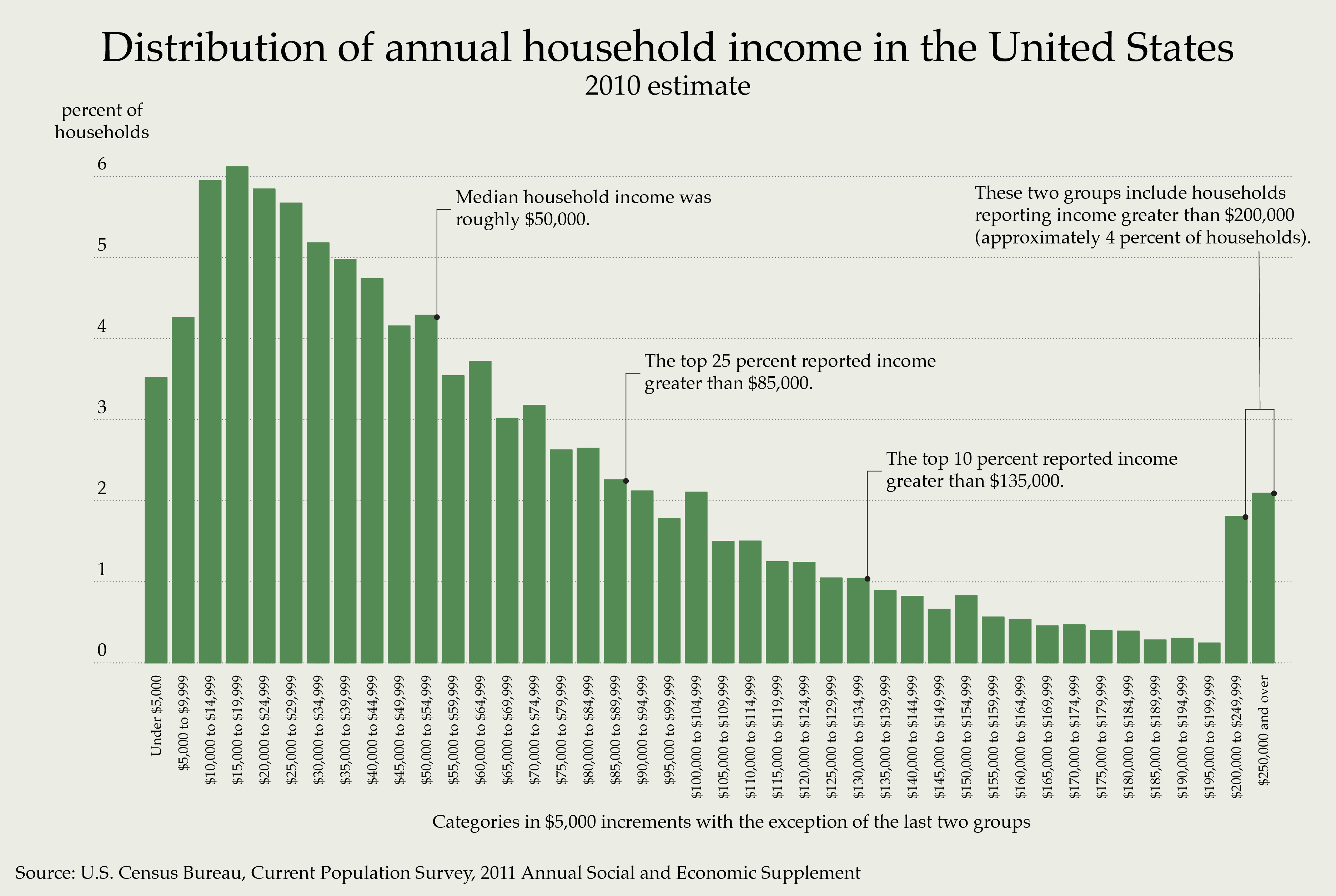
The median of this distribution is about $50,000: half of U.S. households earned more, and half earned less. But the mean is much higher—nearly $100,000—owing both to the overall skewness as well as the long upper tail of the distribution, consisting of a small number of very high earners (the “one percent,” or, at least in this figure, the four percent shown at the far right). Because income distributions tend to be highly skewed and contain huge outliers (like Jeff Bezos or Bill Gates), most economists prefer the median to the mean as a way to measure the “typical” household income.
5.2 Variation
Another important question is, “How spread out are the data points from the typical value?” As we discussed in the lesson on Plots, this variation around the average is usually at least as interesting as the average itself. In fact, I’d encourage you imagine that this full spectrum of variation is the underlying reality, and that any notion of a “typical” or “average” data value—like the notion of an “average American,” with 12.2 years of schooling, 0.9 cars, 0.99 testicles, and 1.01 ovaries—is just an abstraction of that reality.17
In our example, a “typical day” in Rapid City is about 47.3 degrees. But this typical day is actually quite atypical. Some days are much hotter than average; some are much colder; some are about average, but not quite. The number of days that are exactly average is basically zero. Temperature varies. If we want to understand reality, we need the measure that variation. We’ll look at two ways to do this: the standard deviation and the inter-quartile range.
One common way to measure variation is with the standard deviation. The standard deviation answers the question: “by how much do the actual data points tend to deviate from the notionally typical data point?” The higher the number, the more spread out the data points are around their average.
Let’s add the standard deviation to our list of summary statistics that we want to calculate. To do so we use the sd function, like this:
rapidcity %>%
  summarize(avg_temp = mean(Temp),
            median_temp = median(Temp),
            sd_temp = sd(Temp))
## avg_temp median_temp sd_temp
## 1 47.28159 47.6 20.05404In words: the actual days in Rapid City vary from the typical day by about 20 degrees, on average.
To give you a sense of what the standard deviation represents, consider the following table. This shows ten randomly sampled rows of our data set, along with a new column called Temp_deviation. In this column, I’ve calculated the daily deviation: that is, the difference between each day’s actual temperature and the overall average temperature of 47.3 degrees.
| Year | Month | Day | Temp | Temp_deviation |
|---|---|---|---|---|
| 1996 | 6 | 30 | 68.2 | 20.9 |
| 1996 | 11 | 30 | 28.4 | -18.9 |
| 1998 | 12 | 6 | 24.4 | -22.9 |
| 1999 | 12 | 26 | 36.9 | -10.4 |
| 2001 | 9 | 21 | 57.3 | 10.0 |
| 2003 | 7 | 21 | 77.2 | 29.9 |
| 2007 | 4 | 2 | 41.4 | -5.9 |
| 2007 | 5 | 26 | 51.1 | 3.8 |
| 2009 | 3 | 10 | 1.9 | -45.4 |
| 2011 | 1 | 26 | 32.4 | -14.9 |
For example:
- The first row (30 June 1996) shows a temperature of 68.2 degrees F. This is 20.9 degrees above average, and so the
Temp_deviationcolumn shows 20.9.
- The second row (30 November 1997) shows a temperature of 28.4 degrees F. This is 18.9 degrees below average, and so the
Temp_deviationcolumn shows -18.9.
- And so on for the remaining rows.
Some of these deviations are positive, some are negative; some are large, some are small. What the standard deviation measures is, essentially, the average magnitude of these deviations—not just for these 10 rows, but for all 6159 rows of the data set. Said another way, it measures the typical deviation from the average!18
A second conventional measure of variation is called the inter-quartile range, or IQR. This measures the range spanned by the middle half of a data distribution—that is, from the 25th to the 75th percentiles. Let’s add the IQR to our summary table:
rapidcity %>%
  summarize(avg_temp = mean(Temp),
            median_temp = median(Temp),
            sd_temp = sd(Temp),
            iqr_temp = IQR(Temp))
## avg_temp median_temp sd_temp iqr_temp
## 1 47.28159 47.6 20.05404 30.65So in Rapid City, the range from the 25th to the 75th percentile of temperature spans about 31 degrees F.
Some simple advice. Like the median, the IQR is more robust to outliers and heavily skewed data distributions. That’s because it depends only on the middle half of the data, and not what happens in the top or bottom quartile. (If you take a room of 100 school teachers and add Jeff Bezos, the mean and standard deviation of income will change a lot, but the median and IQR will hardly budge.) So if your data distribution is highly skewed or has big outliers in it, you’re usually better off summarizing it with the median and IQR. If not, you’re usually better off with the mean and standard deviation.
5.3 Extremes and quantiles
Another conventional way to summarize a data distribution is to look at the extremes. This is common, for example, in the insurance industry, where they ask questions like, “what’s the worst flood or worst earthquake we might see in a 100-year period?”
The simplest measures of the extremes are the minimum and maximum values we’ve seen before. Let’s add the calculation of these numbers to our summary pipeline, using min and max:
rapidcity %>%
  summarize(avg_temp = mean(Temp),
            median_temp = median(Temp),
            sd_temp = sd(Temp),
            iqr_temp = IQR(Temp),
            min_temp = min(Temp),
            max_temp = max(Temp))
## avg_temp median_temp sd_temp iqr_temp min_temp max_temp
## 1 47.28159 47.6 20.05404 30.65 -19 91.9Minus 19F! Yikes.
Of course, we might think that the min and max are too extreme, to the point of being unrepresentative of the underlying data distribution. I’ll give you an example. By 2021, I’d spent over 15 years of my life in Austin, Texas, and the coldest temperature I’d encountered there was 18 degrees F—until one day in February 2021, when the overnight temperature hit 6 F, shattering both my own personal record low and the state’s power grid. So now when out-of-towners ask me, “What’s the coldest it gets in Austin?” I guess I have to say, “6 degrees.”19 But that figure is actually quite unrepresentative of even the very cold days in an Austin winter—which, as a native Texan, I’d peg at 30 or maybe 35 degrees F, to the derision of my northern friends.
So instead of calculating the min and max temperatures, we might instead want to ask questions about the extremes, but not the very extremes. These kinds of questions are naturally phrased in terms of percentiles. For example:
- What’s the 5th percentile of temperatures? That is, what’s a temperature so cold that only 5% of days in Rapid City are colder?
- What’s the 95th percentile of temperatures? That is, what’s a temperature so hot that 95% of days in Rapid City are colder—or equivalently, only 5% of days are warmer?
To do this, we use the quantile function in R. By convention, quantiles are percentiles expressed on a 0-to-1 scale, so the 5th and 95th percentiles correspond to 0.05 and 0.95 quantiles, respectively. Let’s add these quantiles to our summary pipeline. We’ll also add a step in our pipeline to round these numbers to one decimal place, since this table is getting kinda wide:
rapidcity %>%
  summarize(avg_temp = mean(Temp),
            median_temp = median(Temp),
            sd_temp = sd(Temp),
            iqr_temp = IQR(Temp),
            min_temp = min(Temp),
            max_temp = max(Temp),
            q05_temp = quantile(Temp, 0.05),
            q95_temp = quantile(Temp, 0.95)) %>%
  round(1)
## avg_temp median_temp sd_temp iqr_temp min_temp max_temp q05_temp q95_temp
## 1 47.3 47.6 20.1 30.7 -19 91.9 12.9 77.2So the 5th percentile of temperature in Rapid City is 12.9F, while the 95th percentile is 77.2 F.
We can ask R for any quantiles we want. For example, here are the 25th and 75th percentiles of temperatures in Rapid City, juxtaposed with the inter-quartile range:
rapidcity %>%
  summarize(iqr_temp = IQR(Temp),
            q25_temp = quantile(Temp, 0.25),
            q75_temp = quantile(Temp, 0.75))
## iqr_temp q25_temp q75_temp
## 1 30.65 33.3 63.95Remember that the IQR is precisely the difference between the 75th and 25th percentiles: IQR = 63.95 - 33.3 = 30.65.
5.4 z-scores
Which temperature is more extreme: 50 degrees in San Diego, or 10 degrees in Rapid City? In an absolute sense, of course 10 degrees is a more extreme temperature.20 But what about in a relative sense? In other words, is a 10-degree day more extreme for Rapid City than a 50-degree day is for San Diego? This question could certainly be answered using quantiles, which you’ve already learned how to handle. But let’s discuss a second way: by calculating a z-score for each temperature.
The z-score of some numerical variable \(x\) is the number of standard deviations by which \(x\) is above its mean. (If a z-score is negative, then the corresponding observation is below the mean.)
To calculate a z-score for a number \(x\), we subtract the corresponding mean \(\mu\) and divide by the standard deviation \(\sigma\):
\[ z = \frac{x - \mu}{\sigma} \, . \]
It turns out that the average year-round temperature in San Diego is 63.1 degrees, with a standard deviation of 5.7 degrees. So for a 50-degree day in San Diego, the \(z\)-score is:
\[ z = \frac{50 - 63.1}{5.7} \approx -2.3 \, . \]
Or about 2.3 standard deviations below the mean. On the other hand, Rapid City has a mean temperature of 47.3 degrees and a standard deviation of 20.1 degrees. So for a 10-degree day in Rapid City, the z-score is
\[ z = \frac{10 - 47.3}{20.1} \approx -1.9 \, . \]
Or about 1.9 standard deviations below the mean. Thus a 50-degree day in San Diego is actually more extreme than a 10-degree day in Rapid City! The reason is that temperatures in Rapid City are both colder on average (lower mean) and more variable (higher standard deviation) than temperatures in San Diego.
As this example suggests, z-scores are useful for comparing numbers that come from different distributions, with different statistical properties. It tells you how extreme a number is, relative to other numbers from that same distribution.
Let’s calculate z-scores for each day in Rapid City, using mutate. Really, the worst part about this code is making sure that all the parentheses are balanced! Beyond that, it’s just applying the formula for a \(z\) score:
rapidcity = rapidcity %>%
  mutate(z = (Temp - mean(Temp))/sd(Temp))
Now here are ten random rows of the data set after we’ve calculated the \(z\) scores:
| Year | Month | Day | Temp | z |
|---|---|---|---|---|
| 1996 | 6 | 30 | 68.2 | 1.0431022 |
| 1996 | 11 | 30 | 28.4 | -0.9415354 |
| 1998 | 12 | 6 | 24.4 | -1.1409965 |
| 1999 | 12 | 26 | 36.9 | -0.5176806 |
| 2001 | 9 | 21 | 57.3 | 0.4995708 |
| 2003 | 7 | 21 | 77.2 | 1.4918896 |
| 2007 | 4 | 2 | 41.4 | -0.2932869 |
| 2007 | 5 | 26 | 51.1 | 0.1904061 |
| 2009 | 3 | 10 | 1.9 | -2.2629650 |
| 2011 | 1 | 26 | 32.4 | -0.7420743 |
In general, we think of \(|z| \approx 2\) as the very lower limit of where a data point might be considered “unusual” or “surprising” relative to other numbers from the same distribution. That figure is based on the normal distribution: for normally distributed data, roughly 95% of the data points will fall within 2 standard deviations of the mean. Of course, since most data sets aren’t exactly or even approximately normal, this guideline is very rough indeed. But it at least gives you an order-of-magnitude sense for how to interpret a \(z\)-score. A \(z\)-score of \(\pm 1\), for example, is very typical and not at all surprising. But a \(z\) score of \(\pm 10\) would be a very unusual data point, pretty much no matter how the data are distributed.
Good coders use a combination of strategies to make their code more readable, including line breaks, indentation, informative object names, and commenting.↩︎
The “average American” has more ovaries than testicles because there are slighty more females than males. That’s because females live a bit longer than males, on average.↩︎
This is not quite mathematically precise. The trick in defining the standard deviation is how you ensure the negative and positive deviations don’t cancel each other out in calculating the average. For the formal definition, see pretty much any online tutorial on the concept.↩︎
And about 40 degrees inside without power for a few days.↩︎
I mean compared to what’s comfortable for a person. Clearly if you interpret “absolute” as meaning “compared to the average temperature of the universe,” (2.73 K or -454.76 F), then 50F is the more extreme temperature.↩︎