Lesson 3 Counting

Counting is one of the simplest things you can do with a data set. But it can you get you surprisingly far. I’ve heard it said that data science is mostly plotting and counting things. After all, “How many?” is the most basic quantitative question we can ask about the world. Moreover, from counts, we can get proportions, and from proportions we can estimate probabilities—like, for example, one of the probabilities we’ll estimate below: how likely is a band to play at Austin City Limits Music Festival, given that it played at Lollapalooza earlier that same year?

This lesson is about getting R to do the work of counting for us, so that we can focus on the questions we care about and not the tedious mechanical details of how to answer them. You’ll learn to:

make tables of counts with xtabs.
use prop.table to turn tables of counts into tables of proportions.
use those tables to estimate simple probabilities (including conditional and joint probabilities).
use the pipe operator (%>%) as a way of chaining together computations.

For this lesson, you’ll need to download aclfest.csv, which contains data on some bands that played at several major U.S. music festivals (including our own ACL Fest here in Austin). You’ll also want to create a new R script and name it something (e.g. lesson_tables.R). That way, you can practice the advice from an earlier lesson on Scripts: write statements in scripts, not directly in the console.

3.1 Getting started: ACL Fest

First load the tidyverse library, which we’ll need for just about every R lesson in this book.

library(tidyverse)

Next, use the Import Dataset button to read in aclfest.csv. If you need a reminder on how to accomplish these two key steps, see the previous lessons: Loading a library and Importing a data set.

If you’ve imported the data correctly, you can use the head function to get the first six lines of the file. You should see the following result:

head(aclfest)

##                          band acl bonnaroo coachella lollapalooza outsidelands year
## 1                         ALO   0        0         0            0            1 2008
## 2                     Battles   0        1         1            1            0 2008
## 3                    Bon Iver   0        0         0            0            1 2008
## 4              Flogging Molly   0        0         1            1            0 2008
## 5 Ivan Neville's Dumpstaphunk   0        0         0            0            1 2008
## 6                   Radiohead   0        0         0            1            1 2008

Each entry is either a 1 or a 0, meaning “yes” and “no,” respectively. So, for example, on the 6th line we see an entry of 1 for Radiohead under the lollapalooza column, which means that Radiohead played at Lollapalooza that year.

Let’s make a few simple tables with this data. This will allow us to estimate probabilities like:

How likely is a band in this sample to play Lollapalooza?
How like is a band to play both ACL Fest and Lollapalooza?
How likely is a band to play ACL Fest, given that they played Lollapalooza?

3.2 Simple probabilities

Using xtabs alone

What is P(played Lollapalooza) for a randomly selected band in this sample? To answer this, we’ll use R’s xtabs function to tabulate (i.e. count) the data according to whether a band played Lollapalooza (1) or not (0).

xtabs(~lollapalooza, data=aclfest)

## lollapalooza
##   0   1 
## 800 438

You might be curious about the little tilde (~) symbol in front of lollapalooza. Roughly speaking, ~ means “by” or “according to”—as in, “cross-tabulate BY the lollapalooza variable.”

Remember that, in our table, 1 means yes and 0 means no. So of the 1238 bands (800 + 438) in this sample, 438 of them played Lollapalooza. We can now use R as a calculator to get this proportion:

438/(800 + 438)

## [1] 0.3537964

So about 0.35 (35%). This is a simple illustration of what you might call the “plug-in principle”: if you want to estimate a probability, plug in the corresponding frequency from your data set.

Using prop.table

Simple enough, right? But we can also get R to turn those counts into proportions for us, using the prop.table function. In general, the more work we can get R to do for us, the better.

To do so, we’ll make the same table as before, except that now we’ll save the result in an object whose name we get to choose. (Remember our lesson on Objects.) We’ll call it t1 in the code below, although you could call it something more imaginative, like my_great_lollapalooza_table, if you wanted to.

t1 = xtabs(~lollapalooza, data=aclfest)

Notice that nothing gets printed to the screen when you execute this command. But if you ask R what t1 is, it will show you the same table as before:

t1

## lollapalooza
##   0   1 
## 800 438

OK, so why did we bother to store this table in something called t1? Well, remember the core ideas in data science:

We manage complexity by breaking down complex tasks into simpler tasks, and then linking those simpler tasks together.

That’s exactly what we’re doing here: we’ll take this t1 object we’ve created (the first link our chain) and pass it into the prop.table function (the second link in our chain). This function turns a table of counts (like t1) into a table of proportions, like this:

prop.table(t1)

## lollapalooza
##         0         1 
## 0.6462036 0.3537964

Of course, the answer we get, P(plays Lollapalooza) = 0.354, is the same one we got when we did the division “by hand” (i.e. treating R as a calculator to calculate 438/1238 using numbers we manually peeled off the table created by xtabs).

Using pipes

The above way of doing things—using xtabs creating an “intermediate” object called t1 and then passing t1 into the prop.table function—works just fine. Lots of people write R code this way.

But it turns out there’s a nicer way to accomplish the same task, using a “pipe” (%>%). Pipes allow us to combine multiple operations in a single “pipeline”: that is, a sequential chain of operations, with the result of one operation feeding into the next one.

Here’s an example of a pipeline with just two steps:

xtabs(~lollapalooza, data=aclfest) %>%
  prop.table

## lollapalooza
##         0         1 
## 0.6462036 0.3537964

I tend to think of the pipe symbol (%>%) as meaning “then.” So in English, this code block says:

make a table of counts of the lollapalooza variable in the aclfest data set…
then (%>%) hand off this table of counts to prop.table in order to make a table of proportions.

Pipes make your code easier to easier to write, read, and modify. For a simple calculation like this involving only two steps, the difference is minimal. But for the more complex kinds of calculations we’ll see later in the course, the difference can be substantial.

Piping makes it especially easy to add steps in your pipeline. For example, suppose we wanted to round all numbers to 3 decimal places. This is easily done by adding one more pipe:

xtabs(~lollapalooza, data=aclfest) %>%
  prop.table %>%
  round(3)

## lollapalooza
##     0     1 
## 0.646 0.354

Or in English:

make a table of counts…
then (%>%) turn this into a table of proportions…
then (%>%) round the result to 3 decimal places.

I hope you agree that the rounded table looks nicer. (After all, there are only about 1000 bands in the data set, so proportions beyond the thousandths place are spuriously precise.)

We’ll use pipes a lot in the lessons to come. I like them because they give a very transparent view of the logical flow of steps in a data analysis.

Of course, if you take things to an extreme and try to write everything in your scripts as one long sequence of pipes, it can start to be self-defeating, and your code will be less readable as a result. But for calculations involving somewhere between, say, 2 and 10 steps, pipes are hard to beat from a readability perspective.

One final nice feature of pipes is that, rather than printing the result of a pipeline directly to the screen, you can store the result in an object. Suppose, for example, that we wanted to store our rounded table of probabilities in an object called t2. We’d proceed like this:

t2 = xtabs(~lollapalooza, data=aclfest) %>%
  prop.table %>%
  round(3)

Nothing gets printed when you run this code chunk. However, just as with any user-defined object, t2 is sitting there in memory, waiting to be called upon:

t2

## lollapalooza
##     0     1 
## 0.646 0.354

3.3 Joint probabilities

P(A, B)

Let’s now look at a second question: how likely is a band to play both ACL Fest and Lollapalooza? You might recognize that kind of question as asking for a joint probability of the form P(A, B), or the probability that two events both occur.

We’ll start off by tabulating the bands according to both of the relevant variables: whether they played at ACL (0 or 1), and whether they played at Lollapalooza (0 or 1). This works as follows:

xtabs(~acl + lollapalooza, data=aclfest)

##    lollapalooza
## acl   0   1
##   0 719 361
##   1  81  77

Here you should interpret the + sign as meaning “and,” not in terms of arithmetic. So in English, the code is saying: “cross-tabulate the aclfest data by the acl AND lollapalooza variables.”

The result of calling xtabs gives us some numbers that represent joint frequencies. Remember, for the row and column labels, 1 means yes and 0 means no. So to be specific, the output is telling us that, of the 1238 bands in the data set:

719 played at neither ACL nor Lollapalooza.
81 played at ACL but not Lollapalooza.
361 played at Lollapalooza but not ACL.
77 played at both ACL and Lollapalooza.

From here, we could actually stop and use use a calculator (or use R as a calculator) to work out the relevant joint probability. But as you’ll see, it’s less labor-intensive if we get R to do some of that work for us.

So instead, let’s use prop.table again, to turn those counts into proportions. As with the first example above, we’ll do this using a pipe:

xtabs(~acl + lollapalooza, data=aclfest) %>%
  prop.table %>%
  round(3)

##    lollapalooza
## acl     0     1
##   0 0.581 0.292
##   1 0.065 0.062

These numbers now represent proportions, not counts. Therefore, all the entries in the table sum to 1, rather than to 1238. So to be specific, the table is telling us that:

P(not ACL, not Lollapalooza) = 0.581.
P(not ACL, Lollapalooza) = 0.292
P(ACL, not Lollapalooza) = 0.065
P(ACL, Lollapalooza) = 0.062

And this last number is the answer to the question we set out to answer: the chance that a randomly chosen band from this data set played both ACL and Lollapalooza is P(ACL, Lollapalooza) = 0.062.

P(A or B) and the addition rule

Joint probabilities are also important in calculating probabilities of the form P(A or B), i.e. the probability that one of either A or B, but not necessarily both, occur. Specifically, the addition rule tells us that for any two events A and B,

\[ P(A \mbox{ or } B) = P(A) + P(B) - P(A, B) \]

This equation says that if A and B are two possible outcomes, the probability that either A or B occurs can be built up in three pieces: you add together the individual probabilities for A and B, and then you subtract the probability that A and B both occur, which is like a correction for double-counting.

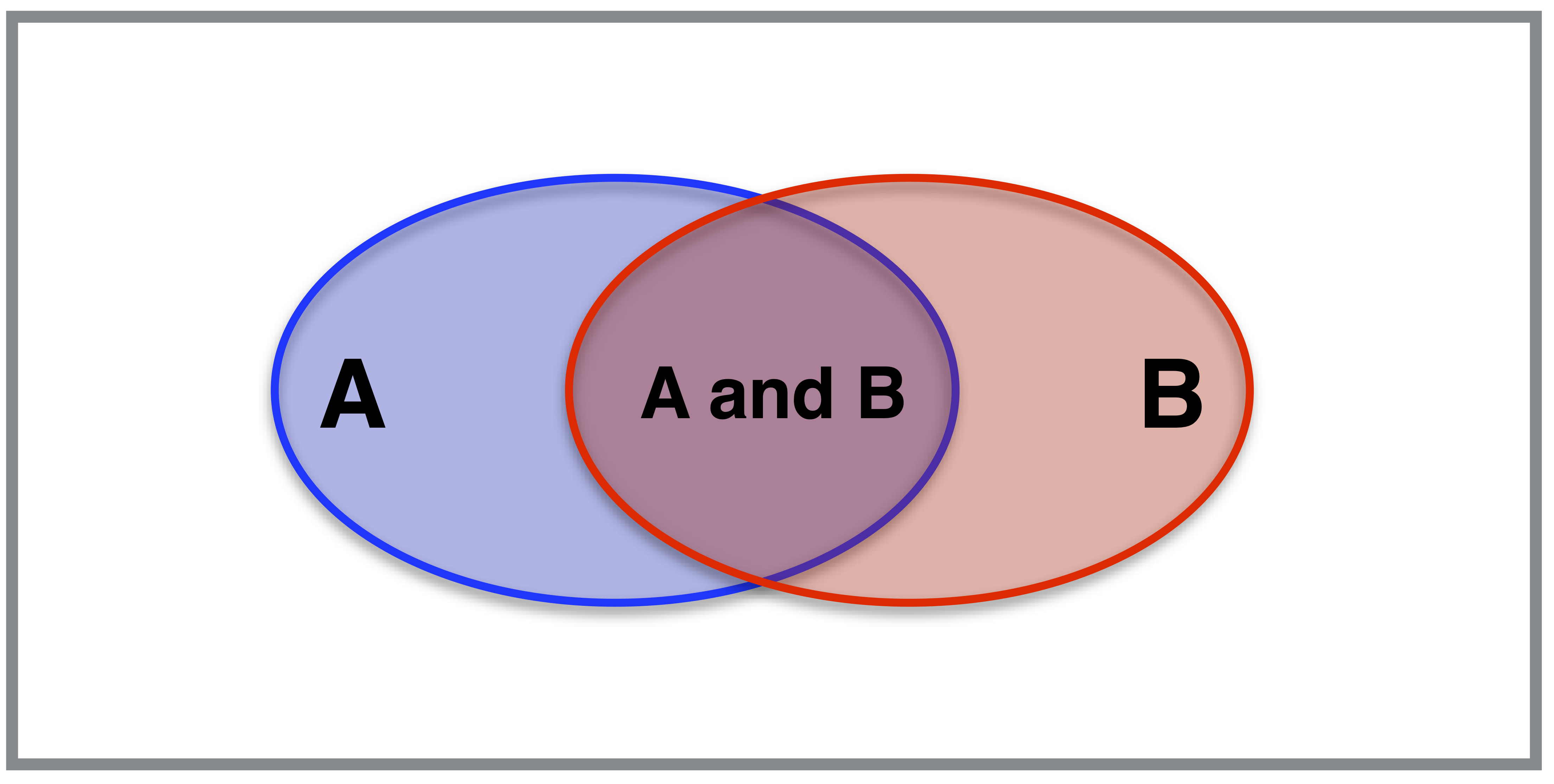
You can visualize this in a Venn diagram like the one above. Imagine throwing darts at this rectangular area. What is P(A or B), the probability that a randomly thrown dart will land either in the blue oval (A) or the red oval (B)? Let’s assume I’m really bad at darts, so that each point in the rectangle is equally likely.

If we assume that the outer rectangle has total area 1, then this probability is just the total area covered by the union of the two ovals. To calculate this area, we can start by adding the areas of the blue oval and red ovals together. But then we’ve double-counted the purple area of overlap: once for the A oval, and once for the B oval. So we have to subtract this area back off, to correct for the double-counting. This leaves us with the area of the A oval plus the area of the B oval, minus the area of their overlap.

For example, let’s use this rule to calculate the probability that a band in our data set played either Bonnaroo or Coachella. For this we need the joint probabilities:

xtabs(~bonnaroo + coachella, data=aclfest) %>%
  prop.table()

##         coachella
## bonnaroo          0          1
##        0 0.33925687 0.40064620
##        1 0.21486268 0.04523425

So the joint probability P(Bonnaroo, Coachella) = 0.045. This is one piece of the addition rule. But what about the other two pieces: P(Bonnaroo) and P(Coachella)? Well, we can get those using what we learned above, in our discussion of Simple probabilities, by calling xtabs for each festival individually:

xtabs(~bonnaroo, data=aclfest) %>%
  prop.table()

## bonnaroo
##         0         1 
## 0.7399031 0.2600969

So P(Bonnaroo) = 0.26. And for Coachella:

xtabs(~coachella, data=aclfest) %>%
  prop.table()

## coachella
##         0         1 
## 0.5541195 0.4458805

This tells us that P(Coachella) = 0.446. So putting these pieces together, we get:

\[ \begin{aligned} P(\mbox{Bonnaroo or Coachella}) &= P(\mbox{Bonnaroo}) + P(\mbox{Coachella}) - P(\mbox{Bonnaroo, Coachella}) \\ &= 0.26 + 0.446 - 0.045 \\ &= 0.661 \end{aligned} \]

I’ll also note a handy labor-saving function called addmargins, which saves you the trouble of making three calls to xtabs:

xtabs(~bonnaroo + coachella, data=aclfest) %>%
  prop.table %>%
  addmargins

##         coachella
## bonnaroo          0          1        Sum
##      0   0.33925687 0.40064620 0.73990307
##      1   0.21486268 0.04523425 0.26009693
##      Sum 0.55411955 0.44588045 1.00000000

addmargins adds the probabilities of the individual events (Bonnaroo and Coachella) in isolation to the margins of the table of joint probabilities:

the bottom row labeled Sum tells us that P(coachella=0) = 0.554 and P(coachella=1) = 0.446.
the right column labeled Sum tells us that P(bonnaroo=0) = 0.740 and P(coachella=1) = 0.260.

So one block of code can get us all three pieces we need in order to do our addition-rule calculation.

3.4 Conditional probabilities

Calculating P(A | B) from data

What is P(played ACL | played Lollapalooza)? Or said in English, what is the conditional probability that a band played ACL, given that they played Lollapalooza? To calculate this, we’ll use the following rule for conditional probabilities:

\[ P(A \mid B) = \frac{P(A,B)}{P(B)} \]

In frequency terms, we can interpret this formula as saying: how often do \(A\) and \(B\) happen together, as a fraction of how often \(B\) happens overall? To estimate this probability using the data, we’ll again tabulate the bands by both the acl and lollapalooza variables:

xtabs(~acl + lollapalooza, data=aclfest)

##    lollapalooza
## acl   0   1
##   0 719 361
##   1  81  77

From this table of counts, we can reason as follows:

There were 361 + 77 = 438 bands that played at Lollapalooza.
Of those 438 bands, 77 played at ACL.
Therefore, P(played ACL | played Lollapalooza) = 77/438.

Let’s use R as a calculator to express this as a decimal number:

77/438

## [1] 0.1757991

So about 0.176.

But as with the previous two examples, it’s much more satisfying to get R to do the work for us. We’ll do this using prop.table again—but this time, with a twist. Pay close attention to the middle line, where we call prop.table:

xtabs(~acl + lollapalooza, data=aclfest) %>%
  prop.table(margin=2) %>%
  round(3)

##    lollapalooza
## acl     0     1
##   0 0.899 0.824
##   1 0.101 0.176

Notice how we added margin=2 inside parentheses in the prop.table() step. What margin=2 does is to tell prop.table that it should calculate proportions conditional on the second variable we named, which was lollapalooza. (Hence margin=2; if you wanted to condition on the first variable you named, which here is acl, you’d type margin=1 instead.)

So having specified that we want to condition on the lollapalooza variable, now we can read off the relevant conditional probabilities directly from the table—no calculator required. Let’s focus on the lollapalooza = 1 column, since this is what we want to condition on (i.e. that a band played Lollapalooza). The numbers in that column tell us that:

P(didn’t play ACL | played Lollapalooza) = 0.824
P(played ACL | played Lollapalooza) = 0.176

And that second number is just the answer we were going for.

Checking independence

In data science, two events are said to be independent if the occurrence of one event does not impact the probability of the occurrence of the other event. Using our conditional probability notation, Events A and B are independent if:

\[ P(A \mid B) = P(A \mid \mbox{not } B) = P(A) \]

This equation means that A and B convey no information about each other: knowing that B occurred does not change the probability of event A when these events are independent. Consider, for example, flipping two fair coins. If we get heads on the first flip, this conveys no information about how likely we are to get heads on second flip: P(heads on flip 2 | heads on flip 1) = P(heads on flip 2 | tails on flip 1) = 0.5. That’s because the two coins are independent.

For two independent events A and B, we can calculate the joint probability that both A and B occur by multiplying the individual probabilities of each event, e.g. P(heads 1 and heads 2) = 0.5*0.5 = 0.25. But we can’t always take this shortcut. For example, we shouldn’t multiply the probability of rain times the probability of high winds to get the probability of both, because rain and high winds convey information about each other: P(rain | high winds) \(\neq\) P(rain | no high winds). Likewise in the case of two siblings. The probability that sibling 2 is colorblind changes if we introduce the information that sibling 1 is colorblind, because colorblindness is a genetic trait.

In general, we might not know whether two events are independent. In that case, we need data! The solution is to check whether B happening seems to change the probability of A happening, or vice versa. That is, we attempt to verify using data whether P(A | B) = P(A | not B) = P(A). These probabilities won’t be exactly alike because of statistical fluctuations, especially with small samples. (We’ll cover this point more in the future lesson on Statistical uncertainty.) But with enough data they should be pretty close if A and B are independent.

For example, in our data on music festivals, suppose we want to check whether playing Coachella is independent of playing Bonnaroo. To check this, we want to see if P(coachella = 1 | bonnaroo = 1) = P(coachella = 1 | bonnaroo = 0)—in other words, whether a band’s playing Bonnaroo affects the probability that the same band plays Coachella. So to check this, let’s form a table of probabilities conditional on the bonnaroo variable:

xtabs(~coachella + bonnaroo, data=aclfest) %>%
  prop.table(margin=2)

##          bonnaroo
## coachella         0         1
##         0 0.4585153 0.8260870
##         1 0.5414847 0.1739130

From this table, it looks like:

P(coachella = 1 | bonnaroo = 1) = 0.17
P(coachella = 1 | bonnaroo = 0) = 0.54

The conclusion is that these two events are clearly not independent. A band that plays Bonnaroo is much less likely to play Coachella in the same year than a band that doesn’t play Bonnaroo.

On the other hand, let’s examine the data on ACL and Outside Lands:

xtabs(~acl + outsidelands, data=aclfest) %>%
  prop.table(margin=2)

##    outsidelands
## acl         0         1
##   0 0.8738050 0.8645833
##   1 0.1261950 0.1354167

From this table, it looks like:

P(acl = 1 | outsidelands = 0) = 0.126
P(acl = 1 | outsidelands = 1) = 0.135

These numbers are not identical, but they’re very close, to the point that we might plausibly explain the difference as a small-sample fluctuation. (Again, we’ll cover the topic of small-sample fluctuations in a future lesson.) So for now, we’d either say that playing ACL and playing Outside Lands look independent of one another, or at the very least that they look nearly independent of one another. Either way, no matter how we choose to phrase our conclusion, it’s clear that whether a band plays Outside Lands conveys little to no information about how likely that band is to play ACL.

Study questions

Use the “aclfest.csv” data set to answer the following questions.

A. What is the joint probability that a band played both Outside Lands and Bonnaroo?
B. What is the conditional probability that a band played Coachella, given that they played ACL Fest? Use pipes (%>%), and write out in English what each line of your code chunk is doing.
Download plays_top50.csv. This file has data on 15,000 users of a music streaming service. The first column is a unique numerical identifier for the user. The remaining columns are for the top 50 artists most frequently streamed by this particular subset of users. The entries in the data frame represent “did play” (1) and “did not play” (0), with 1 meaning that a given user streamed a given artist at least once during the data-collection period. Use this data to answer the following questions:

A. For a randomly selected user, what are P(plays Franz Ferdinand) and P(plays Franz Ferdinand | plays the Killers)?
B. What are P(plays Bob Dylan) and P(plays Bob Dylan | plays the Beatles)?
C. What are P(plays Rihanna) and P(plays Rihanna | plays Kanye West)? Are the events “plays Rihanna” and “plays Kanye West” independent? D. What is P(plays Queen or plays David Bowie)? Hint: for this one you’ll need to know the addition rule, \(P(A \mbox{ or } B) = P(A) + P(B) - P(A,B)\).