Lesson 12 Experiments
12.1 Causal vs. statistical questions
Why have some nations become rich while others have remained poor? Do small class sizes improve student achievement? Does following a Mediterranean diet rich in vegetables and olive oil reduce your risk of a heart attack? Does a green certification (like LEED, for Leadership in Energy and Environmental Design) improve the value of a commercial property?
Questions of cause and effect like these are, fundamentally, questions about counterfactual statements.
For example: “If Colt McCoy had not been injured early in the 2010 National Championship football game, then the Texas Longhorns would have beaten Alabama.” If you judge this counterfactual statement to be true, then you might say that Colt McCoy’s injury caused the Longhorns’ defeat.
Statistical questions, on the other hand, are about correlations. This makes them fundamentally different from causal questions.
- Causal: “If we invested more money in our school system, how much faster would our economy grow?” Statistical: “In looking at data on a lot of countries, how are education spending and economic growth related?”
- Causal: “If I ate more vegetables than I do now, how much longer would I live?” Statistical: “Do people who eat a lot of vegetables live longer, on average, than people who don’t?”
- Causal: “If we hire extra teachers at our school and reduce our class sizes, will our students’ test scores improve?” Statistical: “Do students in smaller classes tend to have higher test scores?”
Causal questions all invoke some kind of hypothetical intervention, where some “treatment” variable is changed and everything else is held equal. Statistical questions, on the other hand, are about the patterns we observe in the real world. And the real world is rarely so simple as the clean hypothetical interventions we might imagine.
For example, suppose we observe that people who eat more vegetables live longer.45 But those same people who eat lots of vegetables probably also tend to exercise more, live in better housing, and work higher-status jobs. These other factors are confounders: they’re associated with vegetable eating, and they also might lead to a longer life-span.
In our hypothetical veggie example, the presence of confounders forces us to ask the question: is it the vegetables that make people live longer, or is it just the other things that vegetable eaters have/are/do? This is a specific version of the general question we’ll address in this chapter: under what circumstances can causal questions be answered using data?
Consider a second example, this one drawn from the pages of USA Today:
A study presented at the Society for Neuroscience meeting, in San Diego last week, shows people who start using marijuana at a young age have more cognitive shortfalls. Also, the more marijuana a person used in adolescence, the more trouble they had with focus and attention. “Early onset smokers have a different pattern of brain activity, plus got far fewer correct answers in a row and made way more errors on certain cognitive tests,” says study author Staci Gruber.
Here the confounder is baseline cognitive performance. Did the smokers get less smart because of the marijuana, or were the less-smart kids more likely to pick up a marijuana habit in the first place? It’s an important question to consider in making drug policy, especially for states and countries where marijuana is legal. But can we know the answer on the basis of a study like this?
You’ve surely heard it said that “correlation does not imply causation.” Obviously. But if not to illuminate causes, what is the point of looking for correlations? Of course correlation does not imply causality, or else playing professional basketball would make you tall. But that hasn’t stopped humans from learning that smoking causes cancer, or that lightning causes thunder, on the basis of observed correlations. The important question is: what distinguishes the good evidence-based arguments from the bad? How can we learn causality from correlation?
It’s not easy, but neither is it impossible. This lesson is about the best way we know how: by running an experiment, also known as a randomized controlled trial (or RCT). The idea of an experiment is simple. If you want to know what would happen if you intervened in some system, then you should intervene and measure what happens. There is simply no better way to establish that one thing causes another.
More specifically, this lesson will teach you the three basic principles of good experimental design:
- Use a control group.
- Block what you can.
- Randomize what you cannot.
12.2 The importance of a control group
The key principle in using experiments to draw causal conclusions is that of a balanced comparison. In this section, we’ll focus on the “comparison” part; in later sections, we’ll focus on the “balanced” part.
In an experiment, a control group is the standard by which comparisons are made. Typically, it’s a group of subjects in an experiment or study that do not receive the treatment under study, but rather are used as a benchmark for the subjects that do receive the treatment. Without a control group, we have no way of knowing whether any changes in the outcome of interest are caused by the treatment, or simply the result of natural variation or pre-existing trends.
To understand the importance of a control group, try to reason through each of the following examples. Could the study in question be used to support a causal claim? Why or why not?
Example 1: You recruit 100 people suffering from cold symptoms. You feed them all lots of oranges, which are full of Vitamin C. Seven days later, 92 out of 100 people are free of cold symptoms. Did the oranges make people better? People generally get better from a cold after several days, without any intervention. It’s impossible to tell whether the oranges had any effect unless you compare orange-eaters (“treatment”) versus non-orange-eaters (“control”).
Example 2: You recruit 100 4th-grade students whose reading skills are below grade level. You get them to enroll them in an after-school reading program at the local library. A year later, their average performance on a reading test has improved by 6%. Did the after-school program help? Kids generally get better at reading over time just by being in school, at least on average. It’s impossible to know how effective the after-school program was unless you compare kids who enrolled in it (“treatment”) versus kids who didn’t enroll (“control).”
Example 3: You conjecture that people will perform worse on a skill-based task when they are in the presence of an observer with a financial interest in the outcome. You recruit 100 subjects and give them time to practice playing a video game that requires them to navigate an obstacle course as quickly as possible. You then instruct each subject to play the game one final time with an observer present. Subjects are randomly assigned to one of two groups. Group 1 is told that the participant and observer will each win $10 if the participant beats a certain threshold time, while Group 2 is told only that the participant will win the prize if the threshold is beaten. At the end of the study, subjects in Group 2 beat the threshold time 9% more often than those in group 1. The study is a true experiment. There is an experimental group and a control group. Moreover, subjects were randomly assigned to either of the groups, ensuring that the only systematic difference between the two groups is the experimental intervention itself. (We’ll talk more about this idea below.) Hence this study could be used to support a causal claim.
The use of a control group is especially important in studying new medical therapies. As one physician reminisces:
One day when I was a junior medical student, a very important Boston surgeon visited the school and delivered a great treatise on a large number of patients who had undergone successful operations for vascular reconstruction. At the end of the lecture, a young student at the back of the room timidly asked, “Do you have any controls?” Well, the great surgeon drew himself up to his full height, hit the desk, and said, “Do you mean did I not operate on half of the patients?” The hall grew very quiet then. The voice at the back of the room very hesitantly replied, “Yes, that’s what I had in mind.” Then the visitor’s fist really came down as he thundered, “Of course not. That would have doomed half of them to their death.” God, it was quiet then, and one could scarcely hear the small voice ask, “Which half?”46
These last two words—“Which half?”—should echo in your mind whenever you are asked to judge the quality of evidence offered in support of a causal claim. Neither a booming authoritative voice nor fancy statistics are a substitute for a controlled experiment.
Some history. The notion of a controlled experiment has been around for thousands of years. The first chapter of the book of Daniel, in the Bible, relates the tale of one such experiment. Daniel and his three friends Hananiah, Mishael, and Azariah arrive in the court of Nebuchadnezzar, the King of Babylon. They enroll in a Babylonian school, and are offered a traditional meat-heavy Babylonian diet. Daniel, however, is a tee-totaling vegetarian; he wishes not to “defile himself with the portion of the king’s meat, nor with the wine which he drank.” So he goes to Melzar, who is in charge of the school, and he asks not to be forced to eat meat or drink wine. But Melzar responds that he fears for Daniel’s health if he were allowed to follow some crank new-age diet. More to the point, Melzar observes, if the new students were to fall ill, “then ye shall make me endanger my head to the king.” Given that Melzar had already been made a eunuch by the king, this fear sounds plausible.
So Daniel proposes a trial straight out of a statistics textbook, designed to compare a diet of beans and water (the “treatment”) with a traditional Babylonian diet (the “control”):
Prove thy servants, I beseech thee, ten days; and let them give us pulse to eat, and water to drink.
Then let our countenances be looked upon before thee, and the countenance of the children that eat of the portion of the king’s meat: and as thou seest, deal with thy servants.
– King James Bible, Daniel 1:12–13.
The King agreed, and the experiment succeeded. When Daniel and his friends were inspected ten days later, “their countenances appeared fairer and fatter in flesh” than all those who had eaten meat and drank wine. Suitably impressed, Nebuchadnezzar brings Daniel and his friends in for an audience, and he finds that “in all matters of wisdom and understanding,” they were “ten times better than all the magicians and astrologers that were in all his realm.”47
Placebos. As for a placebo-controlled trial, in which some of the patients are intentionally given a useless treatment: that idea came much later.48 A placebo, from the Latin placere (“to please”), is any fake treatment designed to simulate the real one. Using a placebo for your control group avoids the possibility that patients might simply imagine that the the latest miracle drug has made them feel better, in a feat of unconscious self-deception called the placebo effect.
Because of placebo effects, we often don’t compare “treatment” with “nothing.” Instead we compare “treatment” with “other treatment.” The “other treatment” might be an actual placebo (e.g. pill with only inactive ingredients, or an injection of nothing but saline). Or it might be some other “status quo” treatment. This kind of experiment is called a placebo-controlled trial.
The first documented placebo-controlled trial in history seems to have taken place in 1784. It was directed by none other than Benjamin Franklin, the American ambassador to the court of King Louis XVI of France. A German doctor by the name of Franz Mesmer had gained some degree of notoriety in Europe for his claim to have discovered a new force of nature that he called, in French, “magnetisme animal,” and which was said to have magical healing powers. The demand for Dr. Mesmer’s services soon took off among the aristocrats of Paris, whom he would “Mesmerize” using a wild contraption involving ropes and magnetized iron rods.
Much to the king’s dismay, his own wife, Marie Antoinette, was one of Mesmer’s keenest followers. The king found the whole Mesmerizing thing a bit dubious, and presumably wished for his wife to have nothing to do with the doctor’s “magnetisme animal.” So he convened several members of the French Academy of Sciences to investigate whether Dr. Mesmer had indeed discovered a new force of nature. The panel included Antoine Lavoisier, the father of modern chemistry, along with Joseph Guillotin, whose own wild contraption was soon to put the King’s difficulties with Mesmer into perspective. Under Ben Franklin’s supervision, the scientists set up an experiment to replicate some of Dr. Mesmer’s prescribed treatments, substituting non-magnetic materials—history’s first placebo—for half of the patients. In many cases, even the patients in the control group would flail about and start talking in tongues anyway. The panel concluded that the doctor’s method produced no effect other than in the patients’ own minds. Mesmer was denounced as a charlatan, although he continues to exact his revenge, via the presence of the word “mesmerize” in the dictionary.
Placebo effects are strikingly common. In fact, for most of human history, placebos were pretty much the only thing doctors had to offer. As Thomas Jefferson once wrote:
One of the most successful physicians I have ever known has assured me that he used more bread pills, drops of coloured water, and powders of hickory ashes, than of all other medicines put together.
Placebos don’t “cure” you in the sense that a doctor would understand the term, but they do genuinely make some people feel better, at least compared with doing nothing. There’s been quite a lot of research on placebos over the years, and we’ve learned a lot about them. In particular, we’ve learned that some placebos are more effective than others. For example:
- Two placebo pills are more effective than one.
- A placebo injection is more effective than a placebo pill.
- A brand-name placebo is more effective than an off-brand placebo.
Some doctors even do placebo surgery. A recent and especially striking example comes from Thomas Freeman, director of the neural reconstruction unit at Tampa General Hospital in Florida. Dr. Freeman performs placebo brain surgery. (You read that correctly.) According to the British Medical Journal,
In the placebo surgery that he performs, Dr Freeman bores into a patient’s skull, but does not implant any of the fetal nerve cells being studied as a treatment for Parkinson’s disease. The theory is that such cells can regenerate brain cells in patients with the disease. Some colleagues decry the experimental method, however, saying that it is too risky and unethical, even though patients are told before the operation that they may or may not receive the actual treatment.49
“There has been a virtual taboo of putting a patient through an imitation surgery,” Dr. Freeman said. “This is the way to start the discussion.” Freeman has performed 106 real and placebo cell transplant operations since 1992. He argues that the medical history is littered with examples of unsafe and ineffective surgical procedures that were not tested against a placebo and resulted in needless deaths, year after year, before doctors abandoned them. (Remember that voice: “which half?”)
12.3 Randomization
The next key principle of good experimental design is randomization, which means randomly assigning subjects to the treatment and control groups. The randomization will ensure that, on average, there are no systematic differences between the two groups, other than the treatment itself. The Latin phrase ceteris paribus, which translates roughly as “with other conditions remaining the same,” is often used to describe such a situation.
The mechanics of randomization look like this:
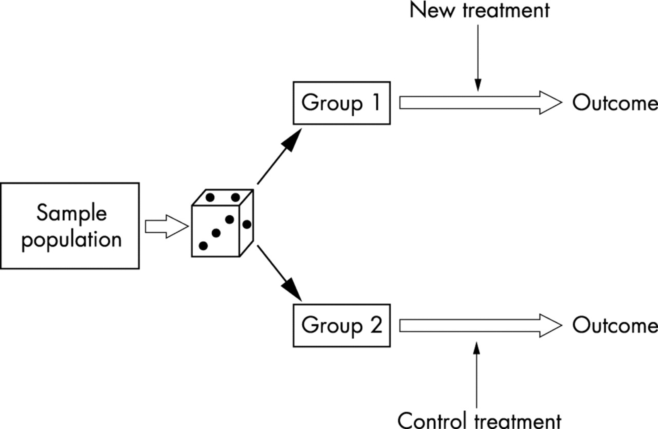
The idea behind randomization is to create treatment and control groups that are balanced with respect to possible confounders. Imagine studying, for example, whether eating more broccoli (“treatment”) improves your blood pressure, versus not eating it (“control”). The challenge here is that lots of other “nuisance” factors drive blood pressure. One example is wealth: wealthier people experience fewer economic and life stresses, potentially lowering their blood pressure. Moreover, it seems reasonable to assume that wealthier people have easier access to fresh foods and vegetables and therefore eat more broccoli than those less wealthy. If that’s true, then broccoli eating will correlate with blood pressure differences, without necessarily causing them.
So if you just observe the blood pressures of broccoli eaters versus non-eaters, you still have a control group. But it’s a really poor control group. In comparing treated with control subjects, you’re implicitly comparing young vs. old, male vs. female, rich vs. poor… You’ve turned all these other nuisance factors that drive blood pressure into confounders: systematic differences between treatment and control groups that also affect the outcome (blood pressure).
On the other hand, what happens if you randomize people to broccoli eating versus no-broccoli eating? Under randomization, sex/age/income differences still affect blood pressure. But all these differences balance out, at least on average: we’d expect the treatment and control groups to have similar characteristics for any possible nuisance factors. Because of randomization, the only systematic difference between broccoli eaters and non-eaters is the treatment, i.e. the broccoli eating itself. So if you see a systematic difference in outcomes, it must have been caused by the broccoli.
Let’s practice applying this principle, by comparing two causal hypotheses arising from two different data sets.
Example 1: effectiveness of chemotherapy. The first comes from a clinical trial in the 1980’s on a then-new form of chemotherapy for treating colorectal cancer, a dreadful disease that has a five-year survival rate of only 60-70% in high-income countries.
The trial followed a simple protocol. After surgical removal of their tumors, patients were randomly assigned to one of two different treatment regimes. Some patients were treated with fluorouracil (the chemotherapy drug, also called 5-FU), while others received no chemotherapy. The researchers followed the patients for many years afterwards and tracked which ones suffered from a recurrence of colorectal cancer.
The outcome of the trial are shown in the table below:
| Surgery + chemo | Surgery alone | |
|---|---|---|
| Recurrence | 119 | 177 |
| No recurrence | 185 | 138 |
| Total | 304 | 315 |
Among the patients who received chemotherapy, 39% (119/304) had a recurring tumor by the end of the study period, compared with 57% of patients (177/315) in the group who received no therapy. The evidence strongly suggests that the chemotherapy reduced the risk of recurrence by a substantial amount.50
We can also type these numbers directly into prop.test if we want to get a confidence interval for the difference in proportions between treatment and control groups:
recurrences = c(119, 177)  # first is treatment, second is control
sample_size = c(304, 315)
prop.test(x=recurrences, n=sample_size)
##
## 2-sample test for equality of proportions with continuity correction
##
## data: recurrences out of sample_size
## X-squared = 17.337, df = 1, p-value = 0.0000313
## alternative hypothesis: two.sided
## 95 percent confidence interval:
## -0.25122803 -0.08968676
## sample estimates:
## prop 1 prop 2
## 0.3914474 0.5619048This command tells R that the number of recurrences (x) in the treatment and control groups were 119 and 177, respectively; while the sample sizes (n) in the two groups were 304 and 315, respectively. The resulting output tells us that the recurrence rate is somewhere between 25% and 9% lower in the treatment group, with 95% confidence. Moreover, we can be confident that this evidence reflects causality, and not merely correlation, because patients were randomly assigned to the treatment and control groups.
It’s worth emphasizing a key fact here. Randomization ensures balance both for the possible confounders that we can measure (like a patient’s age or baseline health status), as well as for the ones we might not be able to measure. This is what makes randomization so powerful, and randomized experiments so compelling. We don’t even have to know what the possible confounding variables are in order for the experiment to give us reliable information about the causal effect of the treatment. Randomization balances everything, at least on average.
Example 2: HIV and circumcision. Next, let’s examine data from a study from the 1990’s conducted in sub-Saharan Africa about HIV, another dreadful disease which, at the time, was spreading across the continent with alarming speed. Several studies in Kenya had found that men who were uncircumcised seemed to contract HIV in greater numbers. This set off a debate among medical experts about the extent to which this apparent association had a plausible biological explanation.
| Circumcised | Not circumcised | |
|---|---|---|
| HIV positive | 105 | 85 |
| HIV negative | 527 | 93 |
| Total | 632 | 178 |
The table above shows some data from one of these studies, which found that among those recruited for the survey, 48% of uncircumcised men (85/178) were HIV-positive, versus only 17% of circumcised men (105/632). The evidence seems to suggest that circumcision reduced a Kenyan man’s chance of contracting HIV by a factor of 3.
But this was not an experiment. Unlike in our first example, the researchers in this second study did not randomize study participants to be circumcised or not. (Imagine trying to recruit participants for that study.) Instead, they merely asked whether each man was circumcised. In the parlance of epidemiology, this was an observational study. It is therefore possible that the observed correlated is due to a confounder, or perhaps multiple confounders. To give two plausible examples, a man’s religious affiliation or age might affect both the likelihood that he is circumcised and the chances that he contracted HIV from unprotected sex. If that were true, the observed correlation between circumcision and HIV status might be simply a byproduct of an imbalanced, unfair comparison, rather than a causal relationship.
We’ll talk more about observational studies later. It is possible to learn about cause and effect without actually running an experiment. It’s just very difficult, because of the possibility of confounders. An experiment, with subjects properly randomized to treatment and control groups, is widely considered the gold standard of evidence in science, and for good reason: randomization balances confounders between the treatment and control groups, even the confounders we don’t know about.
12.4 Blocking
Many interesting research findings come from twins studies, which are designed to settle “nature versus nurture” debates. The classic form of twins study involves identical twins separated since birth and raised by different families; the assumption here is that similarities are more likely to be influenced by genetics, while differences between twins are more likely to be influenced by their environments.
In many cases, the similarities in twins reared apart can be spooky. In one highly publicized case from the 1970s, the identical twins James Lewis and James Springer were separated when they were four weeks old and taken in by different adoptive families. When the twins were reunited for the first time at age 39, it turned out that they shared a lot in common. Both had named their childhood pets “Toy.” Both had married (and divorced) women named Linda, and both had remarried women named Betty. Both were part-time deputy sheriffs in their towns. Both were smokers. Both chewed their fingernails. Both had given their firstborn sons the first name (James) and the same middle name (Alan). They even both took annual road trips with their families to the same three‐block‐long beach in St. Petersburg, Florida. More medically relevant was the first that both Springer and Lewis suffered from a particular type of tension headache that can turn into a migraine. They both manifested their headaches starting at age 18, and they suffered the same symptoms with the same frequency. Scientists had not previously recognized a genetic component to these headaches, but the case of Springer and Lewis made them re-consider.
Most twins studies, of course, are not experiments. However, by way of analogy, they do give us a nice principle to help us reason more effectively about experimental design. The principle is this: in the context of an experiment, the best-case scenario would be to assign treatment and control within a bunch of pairs of identical twins. You’d give one twin the treatment and the other twin the control. If you then noticed that the “treated” twins differed systematically from the “control” twins in some outcome variable, you’d have pretty good evidence of causality. Confounding would be impossible; we’re talking about identical twins, so there would be no systematic differences, other than the treatment itself, that could explain the difference in outcomes.
This principle is called blocking, and it’s an idea that originated in agricultural experiments. Suppose you wanted to test two farming practices, A and B (different seeds, different fertilizers, different cultivation methods, etc.) And suppose you had a big property with a bunch of different areas (“blocks”) that varied enormously in their underlying growing conditions for crops, like this:

Suppose the six boxed-in areas are where you intend to run your experiment. You could simply randomize treatments A and B to these six areas. Then you might get something like this:

This is called complete randomization, i.e. assigning the treatments completely at random. In this case, it looks like we ended up with 2/3 of the B plots on really great land, and 2/3 of the A plots are on not-so-great land. This was just the luck of the draw, but it led to a noticeable imbalance that might lead us to conclude the B is better than A. (This kind of imbalance would less likely to happen with complete randomization if you had more plots of land, but here there are only six.)
A better approach is blocking. You split each area, thereby creating a pair of “identical twins.” You then randomly give half the block treatment A and the other half treatment B, like this:

Now differences in underlying land quality can’t drive the outcome, even by chance: the A’s and the B’s are exactly balanced in terms of where they’re planted.
In general, a block design means arranging of experimental units (people, firms, plots of land, etc.) in groups that are similar to one another. Ideally we would block on any known nuisance variables, like the age or sex of a patient in a clinical trial, or the quality of the plot of land in an agricultural experiment. By blocking on these nuisance variables, we eliminate them as a source of variation due to the randomization process, and we allow variation in the outcome caused by the treatment to stand out more. Of course, we can’t block on everything, so we then randomize the treatment within blocks.
A natural question is: when should we block and when should we randomize? In general, we use blocking to balance confounders that are both known and under the experimenter’s control. We then rely on randomization within blocks to balance all other confounders—that is, those that are either unknown or not under the experimenter’s control. Stated more succinctly: block what you can, randomize what you cannot. Assuming you can actually do it, randomization within blocks is almost always an improvement over complete randomization. Randomization gives us implicit control over confounders; we are hoping that the random assignment hasn’t created large imbalances, even though technically it could, just by chance. (This is why large samples are helpful: with a large sample, it’s much less probable that random assignment would lead to large imbalances.) Blocking, on the other hand, gives us explicit control over confounders. If we block on a nuisance variable, we don’t have to rely on large samples or probability. We know that factor is definitely balanced between treatment and control units, because we balanced it ourselves. (Of course, there might also be confounders we don’t know about, which is why we take the further step of randomizing within blocks.)
Let’s see a couple of real-world examples.
Example 1: Mexico’s Seguro Popular is a program that offers health insurance and regular/preventive medical care to 50 million uninsured Mexicans. But one problem with Seguro Popular, like with all social insurance programs, is actually getting uninsured citizens to enroll and take advantage of free medical care. So the key question studied by a group of researchers in Mexico was: can publicizing Seguro Popular with targeted messaging improve both enrollment and health outcomes?51
The researchers identified 148 “health clusters” willing to participate in an experiment. A health cluster consisted of residents within the catchment area for a single clinic or hospital. They paired the health clusters into 74 groups of 2, ensuring that the facilities in a matched pair were as similar as possible to each other in terms of the socioeconomic and demographic background of their residents. Within each pair, one facility received the treatment and the other the control. For the “treated” areas, the study designers aggressively publicized people’s new rights under Seguro Popular, and they undertook advertising and door-to-door messaging campaigns to get people to enroll in the program. For the “control” areas, they did nothing. The results were striking:
- 44% of residents in treated areas enrolled in the program, and only 4.3% had catastrophic out-of-pocket health-care costs (more than 30% of income).
- But only 7% of residents in the control areas enrolled in the program, while 9.5% had catastrophic out-of-pocket health-care costs.
The researchers could have simply randomized the 148 health clusters to receive the treatment or control, irrespective of their characteristics. By blocking, however, they can do better: they effectively eliminate the possibility of socio-economic or demographic imbalances that might, just by chance, have been introduced by complete randomization.
Example 2: A major priority in education research is to develop cost-effective, scalable interventions that could improve academic outcomes for school-children. To that end, a 2019 study by Yeager et. al. looked at the effectiveness of a so-called “growth mindset” intervention, in the form of a one-hour video. I’ll let the study authors themselves describe this intervention:
[The] growth mindset intervention communicates a memorable metaphor: that the brain is like a muscle that grows stronger and smarter when it undergoes rigorous learning experiences. Adolescents hear the metaphor in the context of the neuroscience of learning, they reflect on ways to strengthen their brains through schoolwork, and they internalize the message by teaching it to a future first-year ninth grade student who is struggling at the start of the year… A growth mindset can motivate students to take on more rigorous learning experiences and to persist when encountering difficulties.
This study had both a treatment and control arm. Again, quoting the authors:
- In the treatment arm, “students were presented with information about neural plasticity that (1) emphasized how brain functions can improve when one confronts new challenges and practices more difficult ways of thinking, and (2) completed writing exercises designed to help students understand and internalize the intervention message by applying the message to their own life and restating the message for a future student.”
- In the control arm, “[Students] did not learn about the brain’s malleability. Instead, they learn about basic brain functions and their localization, for example, the key functions associated with each cortical lobe. The experimental conditions were designed to look very similar so that students’ instructors would remain blind to their condition assignment, and to discourage students from comparing their materials.”
The experiment involved randomization within blocks, as follows. The study involved a random sample of 65 regular public schools in the United States that enrolled 12,490 ninth-graders. Each school was considered a block. Students within schools were then randomized to either treatment or control. The median school had a participation rate of 98%. By using a school as a block, the study team was able to eliminate the possibility of any school-level confounding—for example, the possibility that, just by chance, complete randomization let to more students from richer schools receiving the treatment.
The result of the study was that lower-achieving adolescents earned higher GPAs in core classes at the end of the ninth grade when assigned to the growth mindset intervention, versus the control (about 0.1 GPA points, on average).
12.5 Example: labor market discrimination
Let’s now turn to an example where we actually analyze experimental data ourselves. We’ll look at a famous experiment run by Marianne Bertrand and Sendhil Mullainathan. The researchers sent about 1300 fictitious resumes responding to job ads in Boston and Chicago. To manipulate employer perceptions of race, they used census data on names. For any name, census data tells us how many people in the U.S. have that name, broken down by birth year, sex, and self-identification of race/ethnicity. So the researchers took 36 names: 18 names that were used disproportionately by people self-identifying as White, and another 18 names that were used disproportionately by people self-identifying as Black. They randomized each resume to have either a “Black” or a “White” name, and they then tracked which resumes received a call-back from the employer placing the ad.
The data from this experiment can be found in ResumeNames.csv. Please download this data and import it into RStudio. For our purposes, the two relevant columns are ethnicity, for the randomly assigned ethnicity of the name on the resume; and call, which indicates whether the resume garnered a call-back from the employer placing the ad.
The fundamental question was: do resumes randomized to receive a “White” (coded as cauc, for Caucasian) name receive more call-backs than resumes randomized to receive a “Black” name (coded as afam, for African-American)? The answer, sadly, appears to be yes:
xtabs(~call + ethnicity, data=ResumeNames) %>%
  prop.table(margin=2)
## ethnicity
## call afam cauc
## callback 0.06447639 0.09650924
## no_callback 0.93552361 0.90349076So about 6.4% of Black resumes got a call-back, versus 9.7% of White resumes. That’s a -3.3% difference, with a confidence interval of -4.7% to -1.6%, which we can get via prop.test:
prop.test(call ~ ethnicity, data=ResumeNames)##
## 2-sample test for equality of proportions with continuity correction
##
## data: tally(call ~ ethnicity)
## X-squared = 16.449, df = 1, p-value = 0.00004998
## alternative hypothesis: two.sided
## 95 percent confidence interval:
## -0.04769866 -0.01636705
## sample estimates:
## prop 1 prop 2
## 0.06447639 0.09650924The p-value under the null hypothesis of equal call-back proportions is also tiny: \(4.998 \times 10^{-5}\), or about 0.00005. Remember, other than the names, the resumes were otherwise identical. This is clear and compelling evidence of racial discrimination on the labor market. A 3.3% difference may sound small, but keep in mind that the call-back rate is quite low overall, at only 6.4% for the Black resumes. So in relative terms, the “discrimination effect” was huge: 3.3/6.4 is about 0.5, meaning that White-sounding resumes were nearly 50% more likely in relative terms to receive a call-back than Black-sounding resumes. I’ll let the authors of the study describe this result in their own words:
The results show significant discrimination against African-American names: White names receive 50 percent more callbacks for interviews. We also find that race affects the benefits of a better resume. For White names, a higher quality resume elicits 30 percent more callbacks whereas for African Americans, it elicits a far smaller increase. Applicants living in better neighborhoods receive more callbacks but, interestingly, this effect does not differ by race. The amount of discrimination is uniform across occupations and industries. Federal contractors and employers who list Equal Opportunity Employer’ in their ad discriminate as much as other employers. We find little evidence that our results are driven by employers inferring something other than race, such as social class, from the names. These results suggest that racial discrimination is still a prominent feature of the labor market.
If you’d like a review on how the prop.test command works and why it’s appropriate here, please return to the lesson on Beyond de Moivre’s equation in our chapter on Large-sample inference.
Study questions: experiments
Broccoli
Return to our hypothetical observational study in which we imagine measuring the blood pressure of broccoli eaters (treatment) versus non-broccoli-eaters (control), without randomizing subjects to the two groups. We discussed one potential confounder here: wealth. This was a potential confounder because it seems plausible that wealthier people might have lower blood pressure and eat more broccoli, thereby creating a correlation between broccoli eating and blood pressure that isn’t necessarily causal.
Name two other potential confounders in this observational study, and explain why they’re confounders. Remember, in order to be a confounder, something should affect the outcome of interest (i.e. affect someone’s blood pressure) and also affect the treatment variable of interest (i.e. affect someone’s likelihood of eating broccoli).
Vaccines
Pfizer is conducting an experiment to test a new vaccine, developed to immunize people against a novel strain of the SARS-CoV-2 virus that causes Covid-19. To test the vaccine, Pfizer has 10000 volunteers, 5000 men and 5000 women. The participants range in age from 20 to 70.
- What would a completely randomized experimental design look like in this situation?
- What would randomization within blocks look like, with sex as a blocking variable? Why would this design be better than complete randomization?
Remember the basic mantra of good experimental design! Always use a control group. Block what you can; randomize what you cannot.
True/false
Which of the following statements are true?
- Both completely randomized designs and block designs control for confounding variables, including confounding variables that we don’t even know about.
- In general, we’d expect that a completely randomized design controls for confounding variables better than randomization within blocks.
- A randomized block design does not control for the placebo effect.
- In a block design, participants within each block receive the same treatment.
PREDIMED
Please download the data in predimed.csv. This contains data from the PREDIMED trial, a famous study on heart health conducted by Spanish researchers that followed the lifestyle and diet habits of thousands of people over many years, beginning in 2003. The main purpose of the PREDIMED trial was to assess the effect of a Mediterranean-style diet on the likelihood of someone experiencing a major cardiovascular event (defined by the researchers as a heart attack, stroke, or death from cardiovascular causes). PREDIMED was a true experiment: subjects were randomized either to a Mediterranean diet or a control diet. It also took a long time: the median follow-up time for subjects was nearly five years.
For our purposes the relevant variables in this data set are:
group: which diet the subject was randomized to. There are actually three levels here:Control,MedDiet + VOO, andMedDiet + Nuts. There were actually two versions of the Mediterrean diet, one in which subjects were given nuts to use for snacks, and another in which subjects were given weekly supplementary bottles of extra-virgin olive oil and told that they could use as much as they wanted, however they wanted, in their meals.
event: a yes-or-no variable indicating whether the subject experienced a serious cardiac event during the course of the study.
The question for you to answer is simple: did subjects following a Mediterranean diet experience cardiac events at a lower rate than subjects following the control diet? If so, what is a 95% confidence interval for the difference?
Note: to keep things simple, I recommend collapsing the two versions of the Mediterranean diet into a single MedDietAny category. You can accomplish this easily using ifelse and mutate, like this:
predimed = mutate(predimed,
                  med_diet_any = ifelse(group=="Control", yes="Control", no="MedDietAny"))
I’m not sure if that’s true, but it seems plausible.↩︎
Dr. E. Peacock, University of Arizona. Originally quoted in Medical World News (September 1, 1972). Reprinted pg. 144 of Beautiful Evidence, Edward Tufte (Graphics Press, 2006).↩︎
Well done, Nebuchadnezzar. This realization wouldn’t occur to professional baseball teams for another few millennia.↩︎
See “The Power of Nothing” in the December 12, 2011 edition of The New Yorker (pp. 30–6).↩︎
BMJ. 1999 October 9; 319(7215): 942↩︎
J.A. Laurie et. al. Surgical adjuvant therapy of large-bowel carcinoma: An evaluation of levamisole and the combination of levamisole and fluorouracil. J. Clinical Oncology, 7:1447–56, 1989.↩︎
Public policy for the poor? A randomised assessment of the Mexican universal health insurance programme. King et al, Lancet 373: 9673, pg. 1447-1454 (2009).↩︎