Model fitting
- Rejection sampling and Approximate Bayesian computation
##   Winter  N
## 1   1950 31
## 2   1951 25
## 3   1952 21
## 4   1953 24
## 5   1954 21
## 6   1955 28
# Required functions
calc.lambda <- function(t, t0, gamma, lambda0) {
    lambda0 * exp(gamma * (t - t0))
}
rdunif <- function(n, min, max) {
    sample(min:max, size = n, replace = TRUE)
}

# Algorithm settings
K.tries <- 10^6  # Number of simulated data sets to make
diff <- matrix(, K.tries, 1)  # Vector to save the measure of discrepancy between simulated data and real data
error <- 1000  # Allowable difference between simulated data and real data

# Known random variables and parameters
t0 <- 1949
t <- df1$Winter
z <- df1$N
n <- length(z)

# Unkown random variables and parameters
posterior.samp.parameters <- matrix(, K.tries, 3)  # Matrix to samples of save unknown parameters
colnames(posterior.samp.parameters) <- c("gamma", "lambda0", "p")

y <- matrix(, K.tries, n)  # Matrix to samples of save unknown number of whooping cranes

for (k in 1:K.tries) {
    # Simulate from the prior predictive distribution
    gamma.try <- runif(1, 0, 0.1)  # Parameter model
    lambda0.try <- rdunif(1, 2, 50)  # Parameter model
    lambda.try <- calc.lambda(t = t, t0 = t0, gamma = gamma.try, lambda0 = lambda0.try)  # Mathematical equation for process model
    y.try <- rpois(n, lambda.try)  # Process model
    p.try <- runif(1, 0, 1)  # Prior or data model
    z.try <- rbinom(n, y.try, p.try)  # Data model

    # Record difference between draw of z from prior predictive distribution and
    # observed data
    diff[k, ] <- sum(abs(z - z.try))

    # Save unkown random variables and parameters
    y[k, ] <- y.try
    posterior.samp.parameters[k, ] <- c(gamma.try, lambda0.try, p.try)
}

# Calculate acceptance rate
length(which(diff < error))/K.tries
## [1] 0.01603
# Plot approximate posterior distribution of parameters
library(latex2exp)
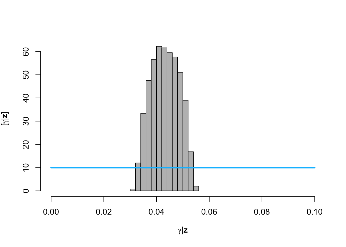
hist(posterior.samp.parameters[which(diff < error), 1], col = "grey", freq = FALSE,
    xlim = c(0, 0.1), main = "", xlab = TeX("$\\gamma  | \\mathbf{z}$"), ylab = TeX("$\\lbrack\\gamma  | \\mathbf{z}\\rbrack$"))
curve(dunif(x, 0, 0.1), col = "deepskyblue", lwd = 3, add = TRUE)

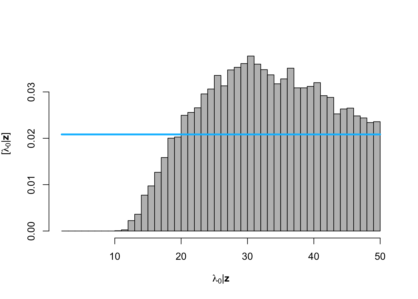
hist(posterior.samp.parameters[which(diff < error), 2], col = "grey", freq = FALSE,
    xlim = c(2, 50), main = "", breaks = seq(2, 50, by = 1), xlab = TeX("$\\lambda_0  | \\mathbf{z}$"),
    ylab = TeX("$\\lbrack\\lambda_0  | \\mathbf{z}\\rbrack$"))
curve(dunif(x, 2, 50), col = "deepskyblue", lwd = 3, add = TRUE)

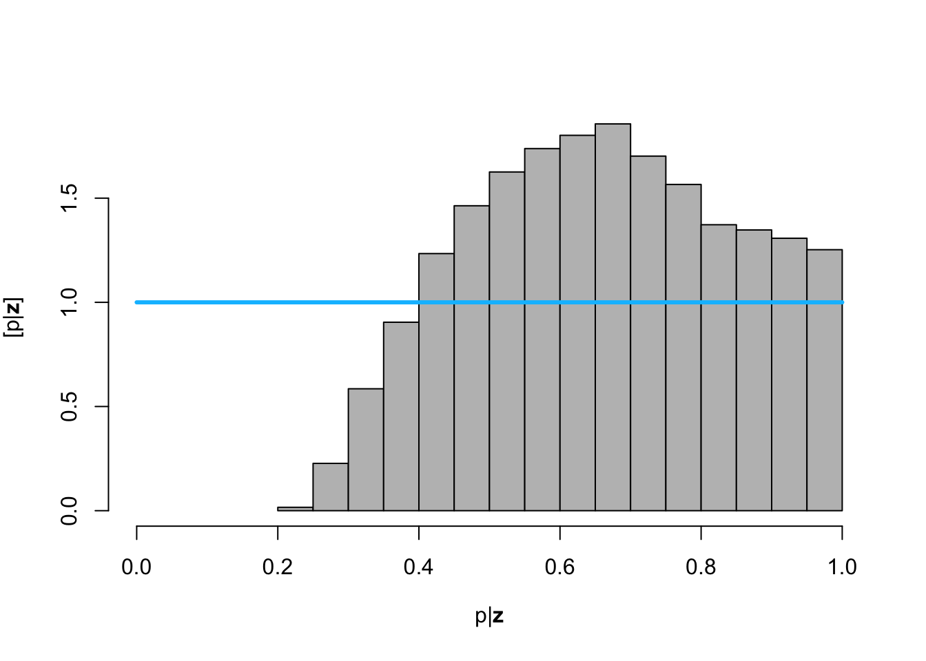
hist(posterior.samp.parameters[which(diff < error), 3], col = "grey", freq = FALSE,
    xlim = c(0, 1), main = "", xlab = TeX("$\\p  | \\mathbf{z}$"), ylab = TeX("$\\lbrack\\p  | \\mathbf{z}\\rbrack$"))
curve(dunif(x, 0, 1), col = "deepskyblue", lwd = 3, add = TRUE)

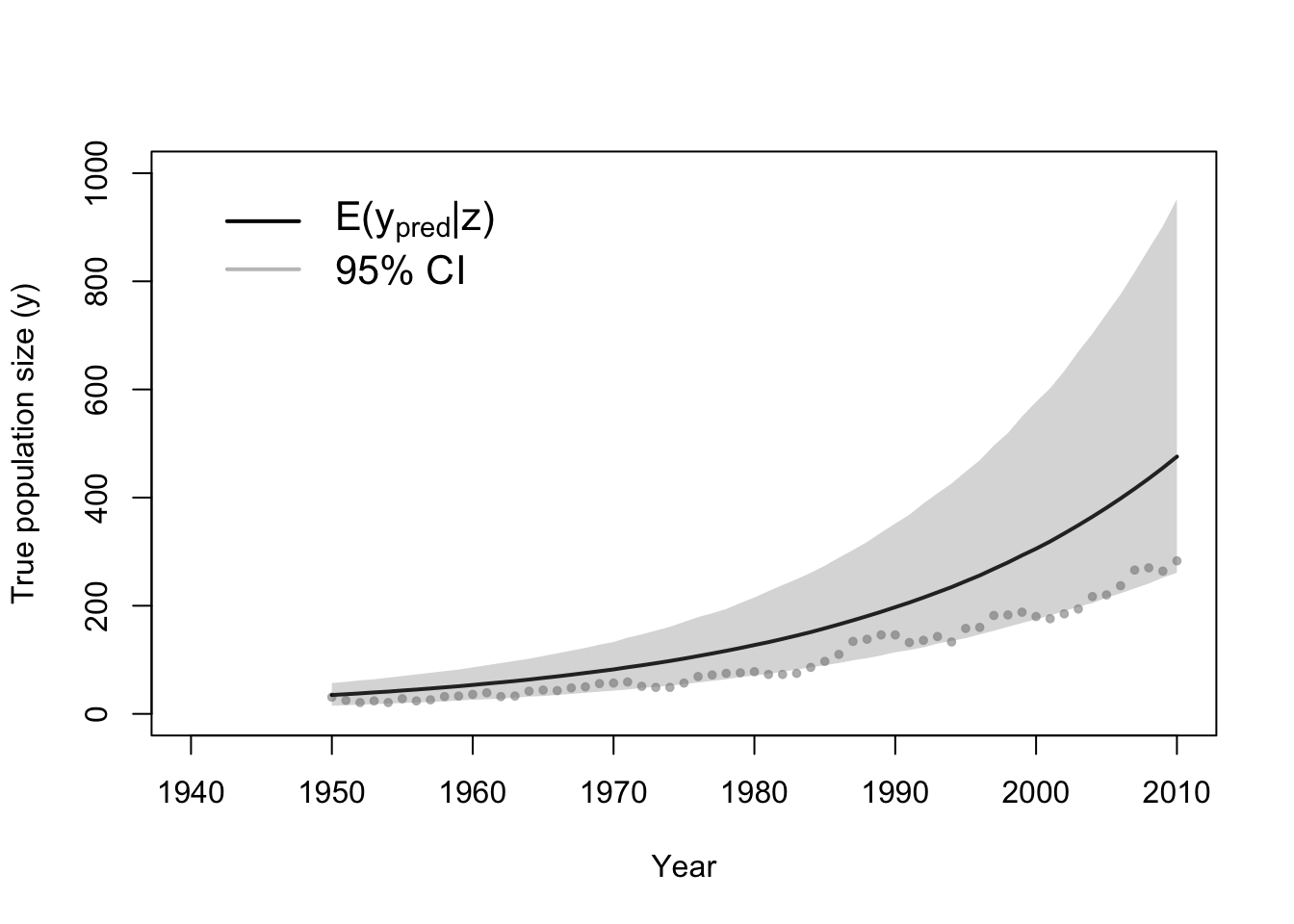
# Plot data (z) and approximate posterior distribution of y
plot(df1$Winter, df1$N, xlab = "Year", ylab = "True population size (y)", xlim = c(1940,
    2010), ylim = c(0, 1000), typ = "b", cex = 0.8, pch = 20, col = rgb(0.7,
    0.7, 0.7, 0.9))
e.y <- colMeans(y[which(diff < error), ])
points(df1$Winter, e.y, typ = "l", lwd = 2)
lwr.CI <- apply(y[which(diff < error), ], 2, FUN = quantile, prob = c(0.025))
upper.CI <- apply(y[which(diff < error), ], 2, FUN = quantile, prob = c(0.975))
polygon(c(df1$Winter, rev(df1$Winter)), c(lwr.CI, rev(upper.CI)), col = rgb(0.5,
    0.5, 0.5, 0.3), border = NA)
legend(x = 1940, y = 1000, cex = 1.3, legend = c(expression("E(" * y[pred] *
    "|" * z * ")"), "95% CI"), bty = "n", lty = 1, lwd = 2, col = c("black",
    rgb(0.5, 0.5, 0.5, 0.5)))

- Recall the goals of the whooping crane study
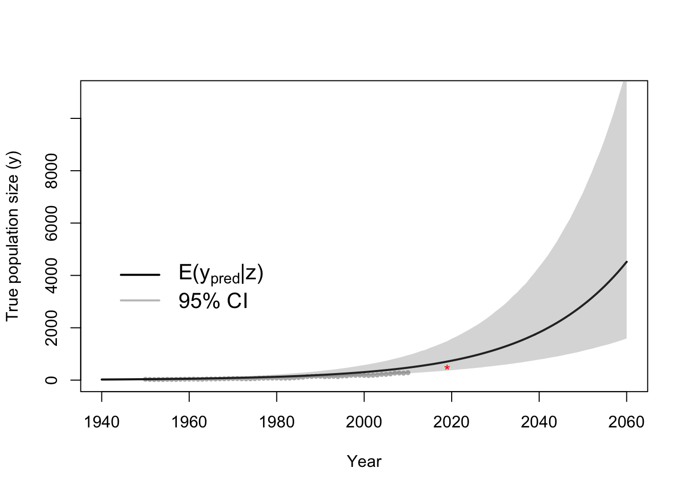
- Predictions and forecasts of the true population size
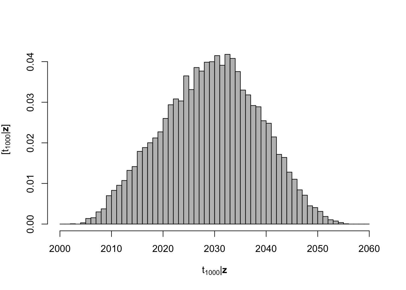
- Statistical inference on the date when the population will be larger than 1000 individuals
- The posterior predictive distribution
- Derived quantity (function of the posterior distribution)
- Live demonstration in R for the whooping crane data example
t.pred <- 1940:2060
n.pred <- length(t.pred)
y.ppd <- matrix(, length(which(diff < error)), n.pred)

for (k in which(diff < error)) {
    gamma <- posterior.samp.parameters[k, 1]
    lambda0 <- posterior.samp.parameters[k, 2]
    lambda.ppd <- calc.lambda(t = t.pred, t0 = t0, gamma = gamma, lambda0 = lambda0)
    y.ppd[which(which(diff < error) == k), ] <- rpois(n.pred, lambda.ppd)
}


# Plot data (z) and approximate posterior predictive distribution of y
plot(df1$Winter, df1$N, xlab = "Year", ylab = "True population size (y)", xlim = c(1940,
    2060), ylim = c(0, 11000), typ = "b", cex = 0.8, pch = 20, col = rgb(0.7,
    0.7, 0.7, 0.9))
e.y.ppd <- colMeans(y.ppd)
points(t.pred, e.y.ppd, typ = "l", lwd = 2)
lwr.CI <- apply(y.ppd, 2, FUN = quantile, prob = c(0.025))
upper.CI <- apply(y.ppd, 2, FUN = quantile, prob = c(0.975))
polygon(c(t.pred, rev(t.pred)), c(lwr.CI, rev(upper.CI)), col = rgb(0.5, 0.5,
    0.5, 0.3), border = NA)
legend(x = 1940, y = 5000, cex = 1.3, legend = c(expression("E(" * y[pred] *
    "|" * z * ")"), "95% CI"), bty = "n", lty = 1, lwd = 2, col = c("black",
    rgb(0.5, 0.5, 0.5, 0.5)))
points(2019, 506, pch = "*", col = "red")

# Derived quantity
date.1000 <- apply(y.ppd, 1, FUN = function(y.ppd) {
    min(t.pred[which(y.ppd >= 1000)])
})
hist(date.1000, col = "grey", freq = FALSE, xlim = c(2000, 2060), main = "",
    breaks = seq(2000, 2060, by = 1), xlab = TeX("$\\t_{1000}  | \\mathbf{z}$"),
    ylab = TeX("$\\lbrack\\t_{1000}  | \\mathbf{z}\\rbrack$"))

- Markov chain Monte Carlo
- One of the most common algorithms used for fitting statistical models in this class
- What to expect in this class
- Algorithm 4.2 (see pg. 169 in Wikle et al. 2019)
- Next time in class
- Other popular approaches for fitting spatio-temporal models
- Computing Bayes: Bayesian Computation from 1763 to the 21st Century (see [Martin et al. 2020] [https://arxiv.org/pdf/2004.06425.pdf])
- Maximum likelihood (non-Bayesian)
- Most spatio-temporal models have to many parameters
- Parameters have discrete and continuous support can be difficult to estimate
- Nuisance parameter are difficult to deal with
- Integrated nested Laplace approximation
- Limited to models that use a Gaussian process as the “process model”
- Rue et al. (2009)
- Hamiltonian Monte Carlo
- Just a different flavor of MCMC
- Stan
- Particle filtering or sequential Monte Carlo
- Statistical emulators
- Approaches that (usually) will not work
- least squares (or similar loss function based estimation approaches)
- machine learning
