2 August 20

2.1 Announcements

Assignment #1 due Friday at 5 pm
- Office hours 9:30 - 10:30 today
PDF/PMF handout -Reading Assignment
- By next Thursday read pgs. 77 - 106 in Wikle et al. (2019)

2.2 Statistical models

What is a model?
- Simplification of something that is real designed to serve a purpose
What is a statistical model?
- Simplification of a real data generating mechanism
- Constructed from deterministic mathematical equations and Probability density /mass functions
- Capable of generating data
What is the purpose of a statistical model
- See section 1.2 on pg. 7 and pg. 77 of Wikle et al. (2019)
- Capable of making predictions, forecasts, and hindcasts
- Enables statistical inference about observable and unobservable quantities
- Reliability quantify and communicate uncertainty
  - Example using simple linear regression

2.3 Matrix review

Column vectors
- $\mathbf{y}\equiv(y_{1},y_{2},\ldots,y_{n})^{'}$
- $\mathbf{x}\equiv(x_{1},x_{2},\ldots,x_{n})^{'}$
- $\boldsymbol{\beta}\equiv(\beta_{1},\beta_{2},\ldots,\beta_{p})^{'}$
- $\boldsymbol{1}\equiv(1,1,\ldots,1)^{'}$
- In R
```
y <- matrix(c(1,2,3),nrow=3,ncol=1)
y
```
```
##      [,1]
## [1,]    1
## [2,]    2
## [3,]    3
```
Matrices
- $\mathbf{X}\equiv(\mathbf{x}_{1},\mathbf{x}_{2},\ldots,\mathbf{x}_{p})$
- In R
```
X <- matrix(c(1,2,3,4,5,6),nrow=3,ncol=2,byrow=FALSE)
X
```
```
##      [,1] [,2]
## [1,]    1    4
## [2,]    2    5
## [3,]    3    6
```
Vector multiplication
- $\mathbf{y}^{'}\mathbf{y}$
- $\mathbf{1}^{'}\mathbf{1}$
- $\mathbf{1}\mathbf{1}^{'}$
- In R
```
t(y)%*%y    
```
```
##      [,1]
## [1,]   14
```
Matrix by vector multiplication
- $\mathbf{X}^{'}\mathbf{y}$
- In R
```
t(X)%*%y
```
```
##      [,1]
## [1,]   14
## [2,]   32
```
Matrix by matrix multiplication
- $\mathbf{X}^{'}\mathbf{X}$
- In R
```
t(X)%*%X
```
```
##      [,1] [,2]
## [1,]   14   32
## [2,]   32   77
```

Matrix inversion

$(\mathbf{X}^{'}\mathbf{X})^{-1}$
In R

solve(t(X)%*%X)

##            [,1]       [,2]
## [1,]  1.4259259 -0.5925926
## [2,] -0.5925926  0.2592593

Determinant of a matrix

$|\mathbf{I}|$
In R

I <- diag(1,3)
I

##      [,1] [,2] [,3]
## [1,]    1    0    0
## [2,]    0    1    0
## [3,]    0    0    1

det(I)

## [1] 1

Quadratic form
- $\mathbf{y}^{'}\mathbf{S}\mathbf{y}$
Derivative of a quadratic form (Note $\mathbf{S}$ is a symmetric matrix; e.g., $\mathbf{X}^{'}\mathbf{X}$ )
- $\frac{\partial}{\partial\mathbf{y}}\mathbf{y^{'}\mathbf{S}\mathbf{y}}=2\mathbf{S}\mathbf{y}$
Other useful derivatives
- $\frac{\partial}{\partial\mathbf{y}}\mathbf{\mathbf{x^{'}}\mathbf{y}}=\mathbf{x}$
- $\frac{\partial}{\partial\mathbf{y}}\mathbf{\mathbf{X^{'}}\mathbf{y}}=\mathbf{X}$

2.4 Distribution theory review

Probability density functions (PDF) and probability mass functions (PMF)
- Normal distribution (continuous support)
- Binomial distribution (discrete support)
- Poisson distribution (discrete support)
- And many more (see handout)

Distributions in R

PDF of the normal distribution $[z|\mu,\sigma^2] = \frac{1}{\sqrt{2\pi\sigma^2}}\textit{e}^{-\frac{1}{2\sigma^2}(z - \mu)^2}$
- $z$ is the random variable
- $\mu$ and $\sigma^2$ are the parameters
PDFs & PMFs in R
- ?dnorm
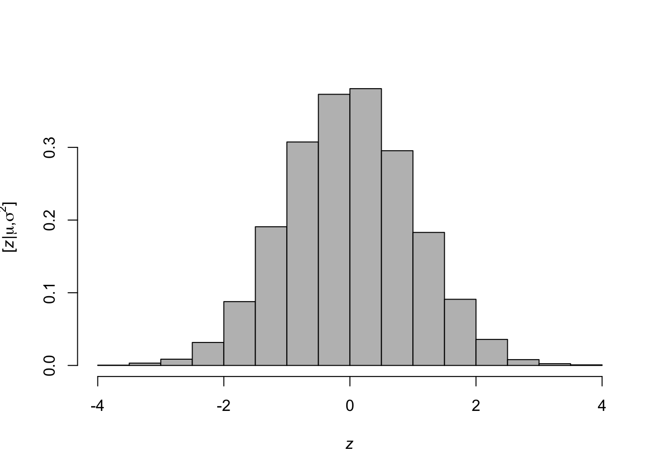
Generate random variables ( $z$ ) from a PDF (e.g., $z_i\sim\text{N}(\mu,\sigma^2)$ )

z <- rnorm(n = 5, mean = 0, sd = 1)
z

## [1]  0.50403669 -1.75030666 -0.43050400  0.01207176 -0.24953909

Histogram representation of a PDF

library(latex2exp)
z <- rnorm(n = 10000, mean = 0, sd = 1)
hist(z,freq=FALSE,col="grey",main = "",
  xlab= TeX('$\\mathit{z}$'),
  ylab = TeX('$\\lbrack\\mathit{z}|\\mu,\\sigma^2\\rbrack$'))

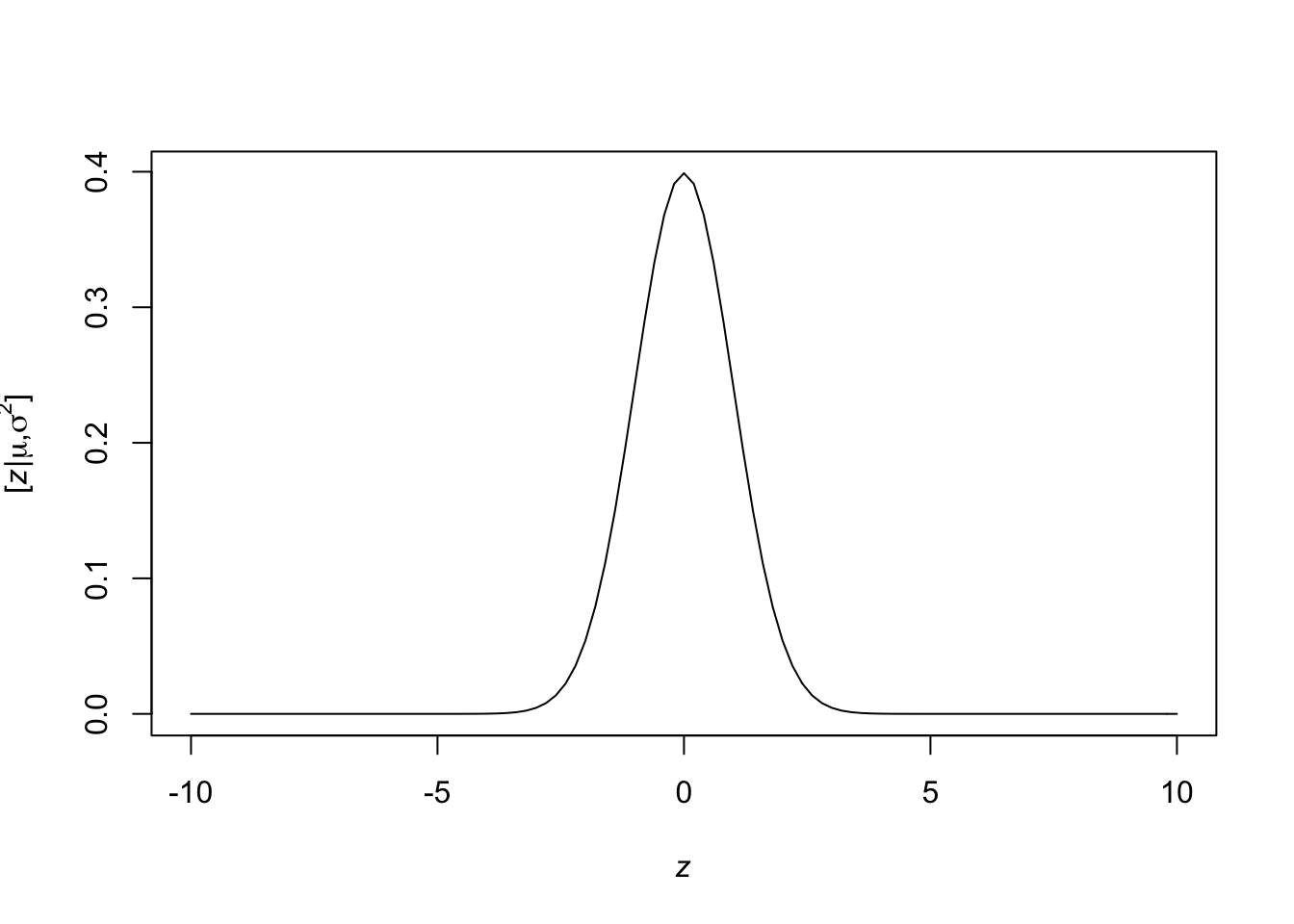
Plot a PDF in R

curve(expr = dnorm(x = x, mean = 0, sd = 1), from = -10, to = 10,
  xlab= TeX('$\\mathit{z}$'),
  ylab = TeX('$\\lbrack\\mathit{z}|\\mu,\\sigma^2\\rbrack$'))

Evaluate the “likelihood” at a given value of the parameters

dnorm(x = 1.759, mean = 0, sd = 1, log = FALSE)

## [1] 0.08492566

Other distributions

rpois(n = 5, lambda = 2)
rbinom(n = 5, size = 10, prob = 0.5)    
runif(n = 5,min = 0,max = 3)
rt(n = 5,df = 1)
rcauchy(n = 5, location = 2, scale = 4)

See stats package for more information

Making your functions for a distribution
- PDF of the exponential distribution $[z|\lambda] = \lambda\textit{e}^{-\lambda z}$
- Make your own function for the PDF of the exponential distribution
```
dexp <- function(z, lambda){lambda*exp(-lambda*z)}
```
- Make your own function to simulate random variables from the exponential distribution using the inverse probability integral transform
```
rexp <- function(n, lambda){
  u <- runif(n)
  -1/lambda*log(1-u)
}
```
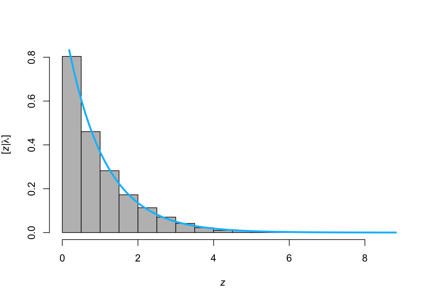
- Make histogram by sampling from rexp() and overlay the PDF using dexp()
```
z <- rexp(n = 10000, lambda = 1)
hist(z,freq=FALSE,col="grey",main = "",
  xlab= TeX('$\\mathit{z}$'),
  ylab = TeX('$\\lbrack\\mathit{z}|\\lambda\\rbrack$'))
curve(expr = dexp(z = x,lambda = 1), from = 0, to = 10, 
  add = TRUE,col = "deepskyblue",lwd = 3)
```
Moments of a distribution
- First moment: $\text{E}(z) = \int z [z|\theta]dz$
- Second central moment: $\text{Var}(z) = \int (z -\text{E}(z))^2[z|\theta]dz$
- Note that $[z|\theta]$ is an arbitrary PDF or PMF with parameters $\theta$
- Example normal distribution $\begin{eqnarray} \text{E}(z) &=& \int_{-\infty}^\infty z\frac{1}{\sqrt{2\pi\sigma^2}}\textit{e}^{-\frac{1}{2\sigma^2}(z - \mu)^2}dz\\&=& \mu \end{eqnarray}$ $\begin{eqnarray} \text{Var}(z) &=& \int_{-\infty}^\infty (z-\mu)^2\frac{1}{\sqrt{2\pi\sigma^2}}\textit{e}^{-\frac{1}{2\sigma^2}(z - \mu)^2}dz\\&=& \sigma^2 \end{eqnarray}$
- Example exponential distribution $\begin{eqnarray} \text{E}(z) &=& \int_{0}^\infty z\lambda\textit{e}^{-\lambda z}dz\\&=& \frac{1}{\lambda} \end{eqnarray}$ $\begin{eqnarray}\text{Var}(z) &=& \int_{0}^\infty (z-\mu)^2\lambda\textit{e}^{-\lambda z}dz\\&=& \frac{1}{\lambda^2} \end{eqnarray}$

2.5 Mathematical model review

Mathematical models are deterministic equations that describe the relationship between input variables and an output variable
Common types of mathematical models used for spatio-temporal statistics
- Linear equations
  - Scalar form: $\mu=\beta_{0}+\beta_{1}x_{1}+\beta_{2}x_{2}+\ldots+\beta_{p}x_{p}$
  - Vector form: $\boldsymbol{\mu}=\beta_{0}+\beta_{1}\mathbf{x}_{1}+\beta_{2}\mathbf{x}_{2}+\ldots+\beta_{p}\mathbf{x}_{p}$
  - Matrix form: $\boldsymbol{\mu}=\mathbf{X}\boldsymbol{\beta}$
- Non-linear equations Scalar form: $\mu = e^{\beta_{0}+\beta_{1}x_{1}+\beta_{2}x_{2}+\ldots+\beta_{p}x_{p}}$
- Difference equations
  - Scalar form: $\mu_{t+1} = \phi\mu_{t}$
- Differential equations
  - Scalar form: $\frac{d\mu(t)}{dt}=\gamma\mu(t)$

2.6 Summary and comments

The material covered today should be review for you
Probability distributions and mathematical models are the building block for most (parametric) statistical models
- Agent-based models simulation models are also widely used but rarely using statistical approaches (Epstein and Axtell 1996; Heard et al. 2015)
Next class meeting we will build our first statistical model!