8 September 10
8.1 Announcements
- No new announcements today
8.2 Extreme precipitation in Kansas
- During the next few lectures, I will demonstrate multiple ways that I would go about meeting the goals in assignment #2
- My process
- Determine the goals of the study
- Exploratory data analysis
- Live demonstration
- The model building process
- 1). Choose appropriate PDFs or PMFs for the data, process, and parameter models
- 2). Choose appropriate mathematical models for the “parameters” or moments of the PDFs/PMFs from step 1.
- 3). Choose an algorithm fit the statistical model to the data
- 4). Make statistical inference (e.g., calculate derived quantities and summarize the posterior distribution)
- Model checking, improvements, validation, and selection (Ch. 6)
- What we will need to learn
- How to use R as a geographic information system
- How to use the hierarchical modeling framework to describe Kriging
- Hierarchical Bayesian model vs. “empirical” hierarchical model
- Specialized language used in spatial statistics (e.g., range, nugget, variogram)
- New general tools from statistics
- Gaussian process
- Metropolis and Metropolis–Hastings algorithms
- Gibbs sampler
8.3 Intro to GIS
- Spatio-temporal data from a statistical and GIS perspective are quite different
- Both disciplines, however, usually classify data based on the spatial support of the “data”
- Data from the GIS perspective
- Using R as a GIS, there are four main types of “data” that we will use.
- Shapefiles
- Raster
- Points
- Using R as a GIS, there are four main types of “data” that we will use.
8.3.1 Shapefiles
- Shapefiles are generally used to represent continuous spatial objects and boundaries
- Examples
- Rivers, streams, and lakes (e.g., National Hydrography Dataset)
- City of Manhattan (link)
- US Census (link)
Example: Shapefiles of each state from the census website
library(rgdal)

url <- "http://www2.census.gov/geo/tiger/GENZ2015/shp/cb_2015_us_state_5m.zip"

tmpdir <- tempdir()
file <- basename(url)
download.file(url, file)
unzip(file, exdir = tmpdir)
shapefile <- paste(tmpdir, "/cb_2015_us_state_5m.shp", sep = "")
ogrListLayers(shapefile)
sf.usa <- readOGR(shapefile, layer = "cb_2015_us_state_5m")

head(sf.usa@data)

sf.kansas <- sf.usa[which(sf.usa@data$NAME == "Kansas"), ]
plot(sf.kansas)
8.3.2 Raster
- Rasters are geographically referenced images (i.e., discrete spatial data)
- Examples
- PRSIM climate data (link)
- CropScape (link)
- Digital Elevation Models (National Elevation Dataset)
- National Land Cover Database (link)
- A few comments about raster files
- Raster files can be very large (e.g., NLCD is 1.1 Gb compressed and 18 Gb uncompressed)
- Raster “data” are usually model based predictions (e.g., PRISM) -Example: 2011 NLCD
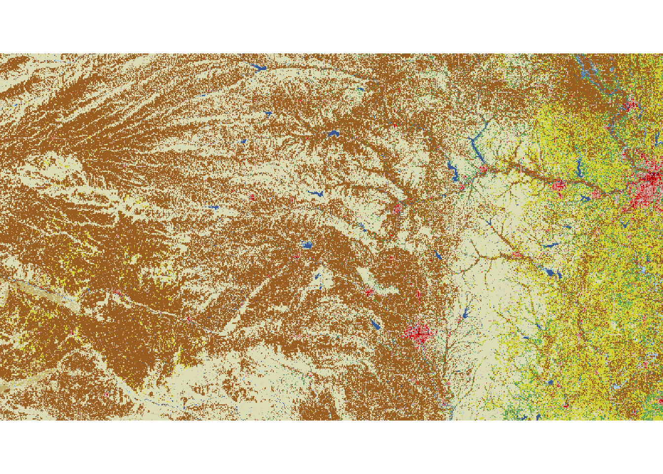
library(raster) # Large file that you may want to save on your computer url.nlcd <- "https://www.dropbox.com/s/rc51iepbo8d3auk/KS_2011_NLCD.img?dl=1" setwd("~/Google Drive/Teaching/Fall 2020/STAT 764 (F2020)/STAT 764 Lecture Notes/Large data sets") url.nlcd <- "KS_2011_NLCD.img" rl.nlcd2011 <- raster(url.nlcd) plot(rl.nlcd2011)## Loading required package: sp# Large file that you may want to save on your computer url.nlcd <- "https://www.dropbox.com/s/rc51iepbo8d3auk/KS_2011_NLCD.img?dl=1" setwd("~/Google Drive/Teaching/Fall 2020/STAT 764 (F2020)/STAT 764 Lecture Notes/Large data sets") url.nlcd <- "KS_2011_NLCD.img" rl.nlcd2011 <- raster(url.nlcd) plot(rl.nlcd2011)
- Transformations and coordinate reference systems
- Not all spatial files have the same coordinate reference systems.
8.3.3 Points
- Point files are created from coordinates (and a corresponding coordinate system)
- Example: Plot location of Dickens Hall
pt.dickens <- data.frame(long = -96.579382, lat = 39.190433)  #Location of Dickens Hall
coordinates(pt.dickens) = ~long + lat
proj4string(pt.dickens) <- CRS("+proj=longlat +datum=WGS84 +no_defs +ellps=WGS84 +towgs84=0,0,0")
pt.dickens <- spTransform(pt.dickens, crs(rl.nlcd2011))

plot(rl.nlcd2011)
plot(sf.kansas, add = TRUE, lwd = 4)
plot(pt.dickens, add = TRUE, col = "green", pch = 20, cex = 3)
Get the landcover type at this location
8.4 Summary
- There are entire courses on what we covered today
- Example (GIS certificate at KSU)
- This is an area that is rapidly developing
- New R packages to automate data downloads
- New sources of data (e.g., UAS)
- Best and most up-to-date resources are usually found be doing a Google search
- Learning how to use R as a GIS can take some time and be frustrating at first