3 August 25

3.1 Announcements

• Make sure you have you PDF/PMF handout handy
• Office hours 9:30 - 10:30 today or by appointment
• Reading assignment
  • By this Thursday read pgs. 77 - 106 in Wikle et al. (2019)
• Pace of the class
  • Poll

3.2 Statistical models

• What is a model?
  • Simplification of something that is real designed to serve a purpose
• What is a statistical model?
  • Simplification of a real data generating mechanism
  • Constructed from deterministic mathematical equations and Probability density /mass functions
  • Capable of generating data
• What is the purpose of a statistical model
  • See section 1.2 on pg. 7 and pg. 77 of Wikle et al. (2019)
  • Capable of making predictions, forecasts, and hindcasts
  • Enables statistical inference about observable and unobservable quantities
  • Reliability quantify and communicate uncertainty

3.3 Bayesian hierarchical models

• During this course we will implement many models using the Bayesian hierarchical framework
  • Today is a crash course on Bayesian statistics
  • It is critical that you understand the concepts that we cover today
  • Study technical note 1.1 on pg. 13 of Spatio-temporal statistics with R
• The Bayesian hierarchical modeling framework

$$\text{Data model:} \;\;[\mathbf{z}|\mathbf{y},\boldsymbol{\theta}_{D}]$$ $$\text{Process model:} \;\;[\mathbf{y}|\boldsymbol{\theta}_{P}]$$ $$\text{Parameter model:} \;\;[\boldsymbol{\theta}]$$

• Given a Bayesian hierarchical model we want the following:
  • The posterior distribution of the parameters $[\boldsymbol{\theta}|\mathbf{z}]$
  • The posterior predictive distribution $[\mathbf{z}_{\text{pred}}|\mathbf{z}]$
• Using Bayes’ theorem… $$[\boldsymbol{\theta}|\mathbf{z}]=\int\frac{[\mathbf{z}|\mathbf{y},\boldsymbol{\theta}][\mathbf{y}|\boldsymbol{\theta}][\boldsymbol{\theta}]}{\int\int\mathbf{[z}|\mathbf{y},\boldsymbol{\theta}][\mathbf{y}|\boldsymbol{\theta}][\boldsymbol{\theta}]d\mathbf{y}d\mathbf{\boldsymbol{\theta}}}d\mathbf{y}$$ $$[\mathbf{z}_{\text{pred}}|\mathbf{z}]=\int\int\mathbf{[z}_{\text{pred}}|\mathbf{y},\boldsymbol{\theta}][\mathbf{y}|\boldsymbol{\theta}][\boldsymbol{\theta}|\mathbf{z}]d\mathbf{y}d\mathbf{\boldsymbol{\theta}}$$

3.3.1 Motivating data example

• Whooping cranes

• Data set

  url <- "https://www.dropbox.com/s/ihs3as87oaxvmhq/Butler%20et%20al.%20Table%201.csv?dl=1"
  df1 <- read.csv(url)
  
  plot(df1$Winter, df1$N, xlab = "Year", ylab = "Population count (z)", xlim = c(1940, 
      2020), ylim = c(0, 300), typ = "b", cex = 0.8, pch = 20, col = rgb(0.7, 
      0.7, 0.7, 0.9))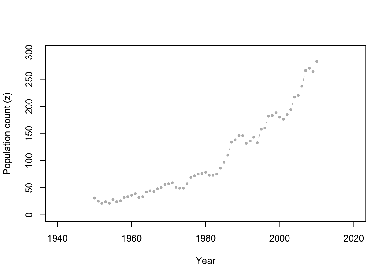

  

• We want to build a statistical model that enables
  • Predictions and forecasts of the true population size
  • Statistical inference on the date when the population will be larger than 1000 individuals
• Points to consider
  • Whooping cranes are counted from an airplane (could some individuals be missed?)
  • Aggregation of a spatio-temporal point pattern
  • Are there any existing models that could work for these data?
  • Anything else?

3.3.2 The data model

• The generic data model is $[\mathbf{z}|\mathbf{y},\boldsymbol{\theta}_{D}]$
  • What is $\mathbf{z}$?
  • What is the process $\mathbf{y}$?
  • What is the support of $\mathbf{z}$ and $\mathbf{y}$?
• What distribution should we use for a data model?
  • Let’s try $[z_{t}|y_{t},p]\equiv\text{Binomial}(y_{t},p)$
  • Live demonstration in R
• What mathematical model should we use?
  • How would the mathematical model control the moments of the PDF/PMF of the data model?

3.3.3 The process model

• The generic process model is $[\mathbf{y}|\boldsymbol{\theta}_{P}]$
• What distribution should we use for a process model?
  • What is the support of $\mathbf{y}$?
  • Let’s try $[z_{t}|\lambda_{t}]\equiv\text{Poisson}(\lambda_{t})$
  • Live demonstration in R
• What mathematical model should we use?
  • Study technical section 1.2 (pgs. 7-10) of Spatio-temporal statistics with R
  • Descriptive mathematical model: $$\lambda_{t} = e^{\beta_0+\beta_{1}t}$$
  • Dynamic mathematical model: The number of whooping cranes at any given time ($t$) can be constructed by $$\begin{equation} \lambda(t+\Delta t)=\lambda(t)+b(t)-d(t) . \tag{3.1} \end{equation}$$ At time $t$, let the births equal $b(t)=\beta\Delta t\lambda(t)$ and deaths equal $d(t)=\alpha\Delta t\lambda(t)$. Then write (3.2) as $$\begin{equation} \lambda(t+\Delta t)=\lambda(t)+\beta\Delta t\lambda(t)-\alpha\Delta t\lambda(t). \tag{3.2} \end{equation}$$ Now define the growth rate as $\gamma=\beta-\alpha$ and rewrite (3.2) as $$\begin{equation} \lambda(t+\Delta t)=\lambda(t)+\gamma\Delta t\lambda(t). \tag{3.3} \end{equation}$$ Next write (3.3) as $$\begin{equation} \frac{\lambda(t+\Delta t)-\lambda(t)}{\Delta t}=\gamma\lambda(t) \tag{3.4} \end{equation}$$ Take the limit of (3.4) as $\Delta t\rightarrow0$. $$\begin{equation} \lim_{\Delta t\rightarrow0}\frac{\lambda(t+\Delta t)-\lambda(t)}{\Delta t}=\gamma\lambda(t) \tag{3.5} \end{equation}$$ Finally replace $\lim_{\Delta t\rightarrow0}\frac{\lambda(t+\Delta t)-\lambda(t)}{\Delta t}$ in (3.5) with the differential operator to get $$\begin{equation} \frac{d\lambda(t)}{dt}=\gamma\lambda(t). \tag{3.6} \end{equation}$$ The analytical solution to (3.6) is $$\begin{equation} \lambda(t)=\lambda_{0}e^{\gamma (t-t_0)}\ \tag{3.7} \end{equation}$$

3.3.4 The parameter model

• The final step is to specify PDFs/PMFs for the parameters
  • In what follows we will use the Binomial data model and Poisson process model (with the exponential growth mathematical model)
  • What parameter models should we use?

3.3.5 Simulating data from the prior predictive distribution

• The prior predictive distribution is capable of providing predictions/forecasts without the use of any data
  • Other fields call this “simulation modeling” or a “sensitivity analysis”
  • It is basically data free statistics (i.e., prediction, forecasts, and inference is 100% assumption driven)
  • Used as a form of model (assumption) checking in Bayesian statistics
  • Super easy to do and helps us “prototype” our statistical model before we put in any more work
• Live demonstration in R

3.3.6 Model fitting

• Class discussion
• We will cover this in future lectures

3.4 Summary and comments

• Bayesian hierarchical modeling framework is incredibly flexible
  • Motivated by a data set or practical problem, you can build your own “custom” statistical models
  • You can always “turn the Bayesian crank” for whatever model you develop (with some warnings of course!)
• Practice the process of model specification (what we did today in class) at home on a different data set