20 October 22
20.1 Announcements
- All proposals have been graded and returned with comments (check your email)
- Redo of assignment 2 and 3
- Q & A for assignment 4
20.2 Mechanistic spatio-temporal models for trajectories
- Descriptive vs. mechanistic models for trajectories
- What are the goals?
- Prediction
- Inference
- Mechanistic understanding
- Brownian motion
- Animations from Wikipedia
- A model for trajectories based on Brownian motion can be written as \[\mathbf{y}(t_{i})=\mathbf{y}(t_{0})+\lim_{\Delta t\rightarrow0}\sum_{j=0}^{i}\boldsymbol{\varepsilon}(t_{j})\] where \(\boldsymbol{\varepsilon}(t_{j})\sim\text{N}(\mathbf{0},\sigma^{2}_{y}\Delta\mathit{t}\mathbf{I})\).
- Alternatively Brownian motion can be written as a stochastic integral equation
- Example simulating Brownian motion in R
t.obs <- seq(0, 300, by = 1)
sigma2.y <- 1

set.seed(1309)
e1 <- rnorm(length(t.obs), 0, (diff(t.obs) * sigma2.y)^0.5)
e2 <- rnorm(length(t.obs), 0, (diff(t.obs) * sigma2.y)^0.5)

y <- matrix(, length(t.obs), 2)

# Starting location
y[1, 1] <- 0
y[1, 2] <- 0

for (t in 1:(length(t.obs) - 1)) {
    y[t + 1, 1] <- y[t, 1] + e1[t]
    y[t + 1, 2] <- y[t, 2] + e2[t]
}

# Plot locations
plot(y[, 1], y[, 2], xlab = expression(y[1]), ylab = expression(y[2]), typ = "b",
    pch = "*")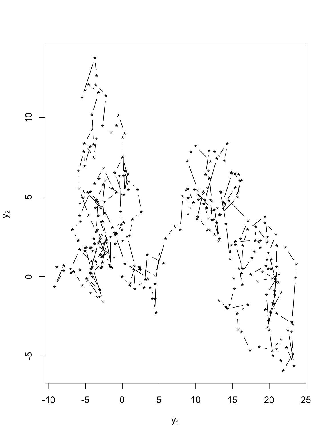
# Plot time series of locations
par(mfrow = c(2, 1))
plot(y[, 1], xlab = "Time", ylab = expression(y[1]), typ = "b", pch = "*")
abline(a = 0, b = 0)
plot(y[, 2], xlab = "Time", ylab = expression(y[2]), typ = "b", pch = "*")
abline(a = 0, b = 0)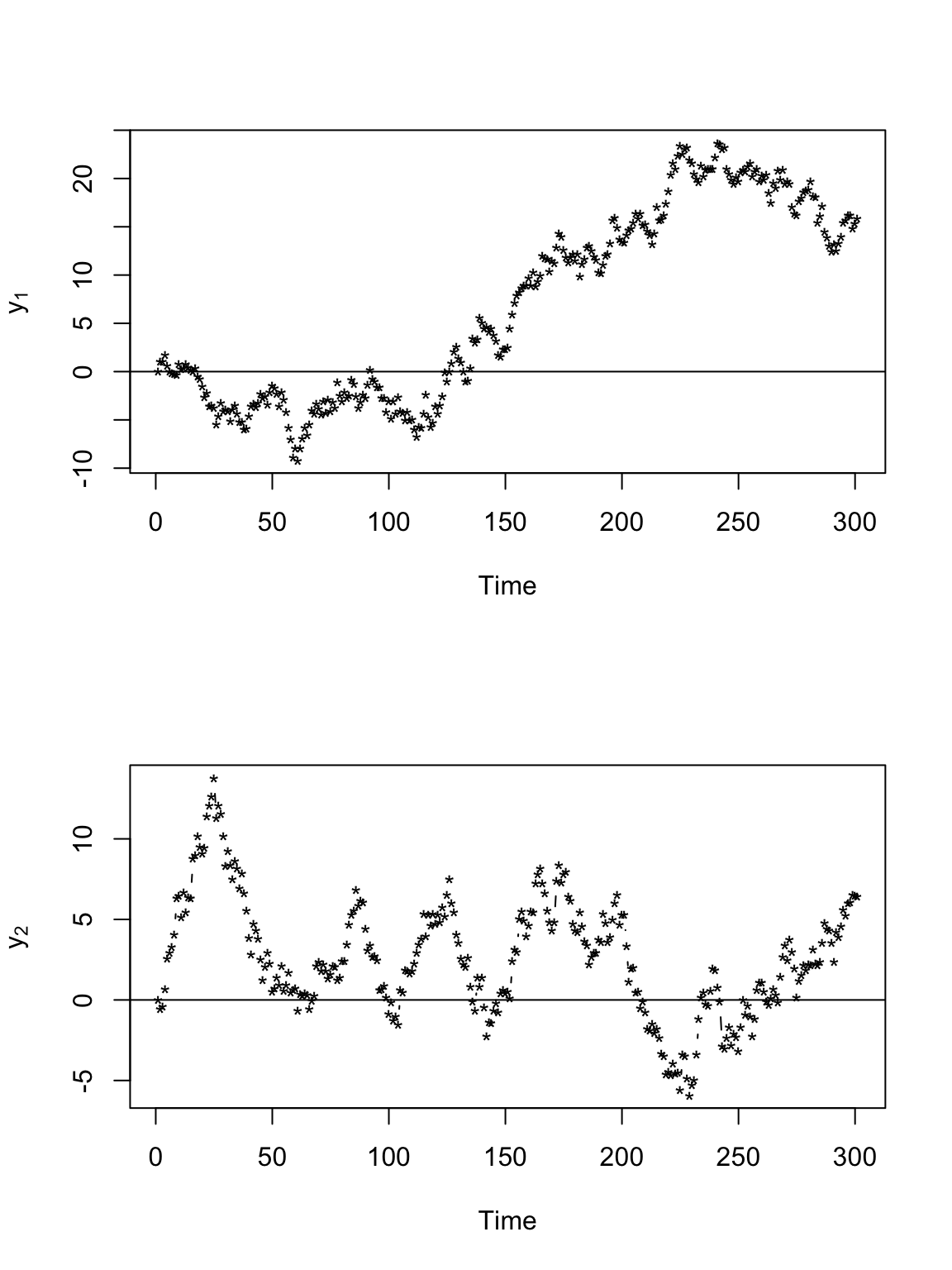
Example simulating from an AR(1) process in R
t.obs <- seq(0, 300, by = 1)
sigma2.y <- 1
alpha <- 0.8

set.seed(1309)
e1 <- rnorm(length(t.obs), 0, (diff(t.obs) * sigma2.y)^0.5)
e2 <- rnorm(length(t.obs), 0, (diff(t.obs) * sigma2.y)^0.5)

y <- matrix(, length(t.obs), 2)

# Starting location
y[1, 1] <- 0
y[1, 2] <- 0

for (t in 1:(length(t.obs) - 1)) {
    y[t + 1, 1] <- alpha * y[t, 1] + e1[t]
    y[t + 1, 2] <- alpha * y[t, 2] + e2[t]
}

# Plot locations
plot(y[, 1], y[, 2], xlab = expression(y[1]), ylab = expression(y[2]), typ = "b",
    pch = "*")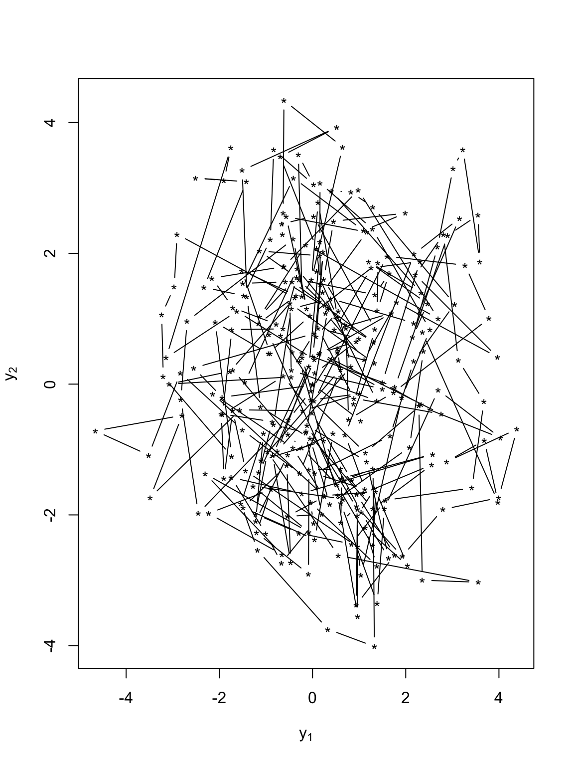
# Plot time series of locations
par(mfrow = c(2, 1))
plot(y[, 1], xlab = "Time", ylab = expression(y[1]), typ = "b", pch = "*")
plot(y[, 2], xlab = "Time", ylab = expression(y[2]), typ = "b", pch = "*")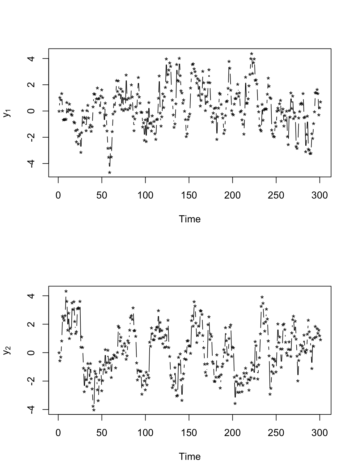
- Mechanistic models for velocity
- All models so far have modeled position directly
- Given an initial starting point and a velocity, we can calculate location
- Velocity that is white-noise (same as position that is Brownian motion)
t.obs <- seq(0, 300, by = 1)
sigma2.y <- 1

set.seed(1309)
e1 <- rnorm(length(t.obs), 0, (diff(t.obs) * sigma2.y)^0.5)
e2 <- rnorm(length(t.obs), 0, (diff(t.obs) * sigma2.y)^0.5)

y <- matrix(, length(t.obs), 2)
v <- matrix(, length(t.obs), 2)

# Starting location
y[1, 1] <- 0
y[1, 2] <- 0

for (t in 1:(length(t.obs) - 1)) {

    # Velocity
    v[t, 1] <- e1[t]
    v[t, 2] <- e2[t]

    # Position
    y[t + 1, 1] <- y[t, 1] + v[t, 1]
    y[t + 1, 2] <- y[t, 2] + v[t, 2]
}

# Plot locations
plot(y[, 1], y[, 2], xlab = expression(y[1]), ylab = expression(y[2]), typ = "b",
    pch = "*")
# Plot time series of locations
par(mfrow = c(2, 1))
plot(y[, 1], xlab = "Time", ylab = expression(y[1]), typ = "b", pch = "*")
abline(a = 0, b = 0)
plot(y[, 2], xlab = "Time", ylab = expression(y[2]), typ = "b", pch = "*")
abline(a = 0, b = 0)
# Plot time series of velocity
par(mfrow = c(2, 1))
plot(v[, 1], xlab = "Time", ylab = expression(v[1]), typ = "b", pch = "*")
abline(a = 0, b = 0)
plot(v[, 2], xlab = "Time", ylab = expression(v[2]), typ = "b", pch = "*")
abline(a = 0, b = 0)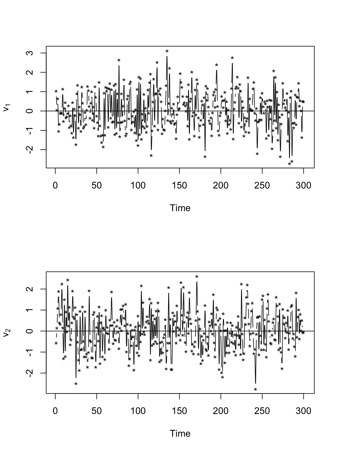
Velocity that is AR(1)
t.obs <- seq(0, 300, by = 1)
sigma2.y <- 1
alpha <- 0.8

set.seed(1309)
e1 <- rnorm(length(t.obs), 0, (diff(t.obs) * sigma2.y)^0.5)
e2 <- rnorm(length(t.obs), 0, (diff(t.obs) * sigma2.y)^0.5)

y <- matrix(, length(t.obs), 2)
v <- matrix(, length(t.obs), 2)

# Starting location
y[1:2, 1] <- 0
y[1:2, 2] <- 0

# Starting velocity
v[1, 1] <- 0
v[1, 2] <- 0

for (t in 2:(length(t.obs) - 1)) {

    # Velocity
    v[t, 1] <- alpha * v[t - 1, 1] + e1[t]
    v[t, 2] <- alpha * v[t - 1, 2] + e2[t]

    # Position
    y[t + 1, 1] <- y[t, 1] + v[t, 1]
    y[t + 1, 2] <- y[t, 2] + v[t, 2]
}

# Plot locations
plot(y[, 1], y[, 2], xlab = expression(y[1]), ylab = expression(y[2]), typ = "b",
    pch = "*")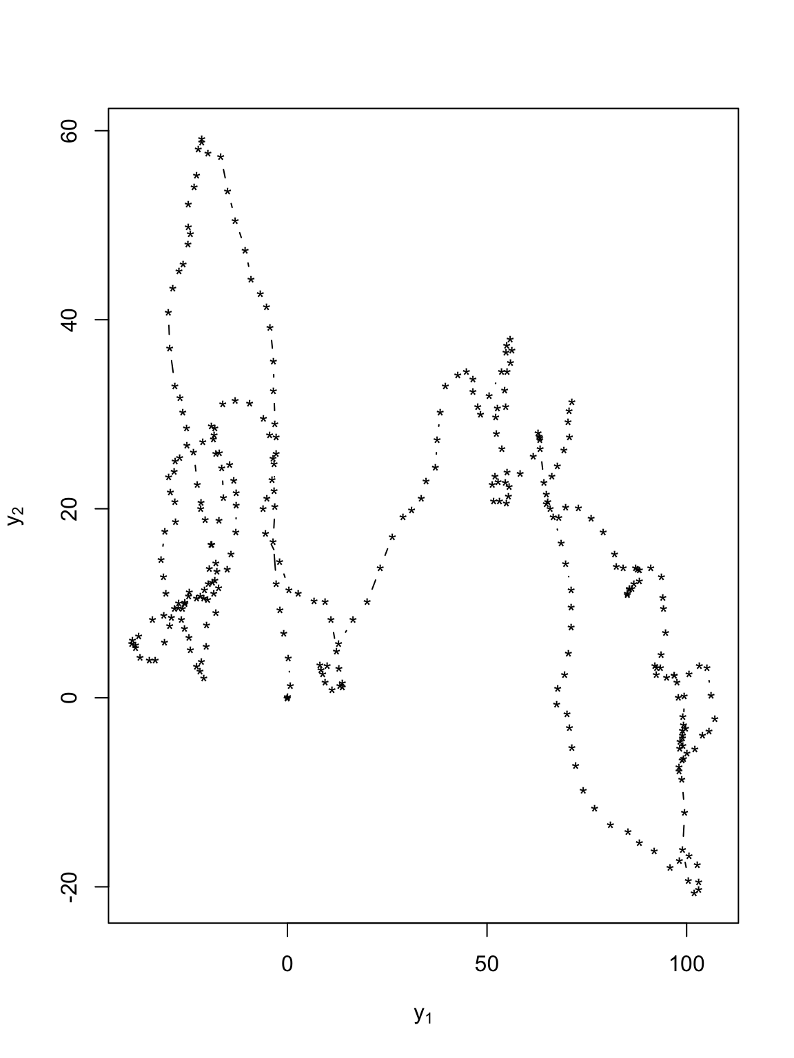
# Plot time series of locations
par(mfrow = c(2, 1))
plot(y[, 1], xlab = "Time", ylab = expression(y[1]), typ = "b", pch = "*")
abline(a = 0, b = 0)
plot(y[, 2], xlab = "Time", ylab = expression(y[2]), typ = "b", pch = "*")
abline(a = 0, b = 0)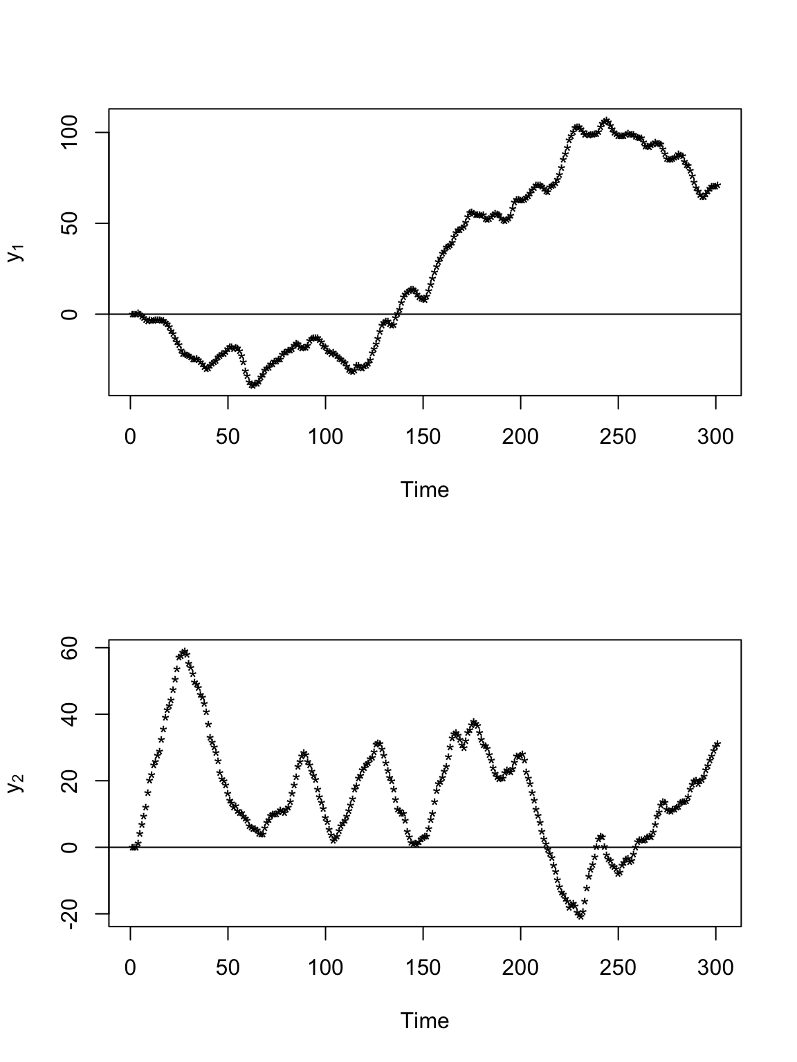
# Plot time series of velocity
par(mfrow = c(2, 1))
plot(v[, 1], xlab = "Time", ylab = expression(v[1]), typ = "b", pch = "*")
abline(a = 0, b = 0)
plot(v[, 2], xlab = "Time", ylab = expression(v[2]), typ = "b", pch = "*")
abline(a = 0, b = 0)
- Measurement error
- Is \(\mathbf{y}(t_{i})\) recorded without error?
- Example
- Based on Bayesian linear model
- Velocity that is Brownian motion
library(plotKML)
library(lubridate)
library(rgdal)
library(raster)
library(gdata)
library(fields)
library(MASS)

url <- "https://www.dropbox.com/s/ulbn9m3uyz6d0a5/Abilene_Running.gpx?dl=1"
# ogrListLayers(url)
pt.marathon <- readOGR(url, "track_points")
## OGR data source with driver: GPX ## Source: "https://www.dropbox.com/s/ulbn9m3uyz6d0a5/Abilene_Running.gpx?dl=1", layer: "track_points" ## with 2095 features ## It has 27 fields# head(data.frame(pt.marathon)) # Change date/time to class 'POSIXct' pt.marathon$time <- ymd_hms(pt.marathon$time, "%Y-%m-%d %H:%M:%S", tz = "America/Chicago")[-2096] # Drop all extra variables pt.marathon <- pt.marathon[1:122, 5] # Assign coordinate reference system to pt.marathon and then project to UTM proj4string(pt.marathon) <- "+proj=longlat +zone=14 +datum=WGS84" pt.traj <- spTransform(pt.marathon, CRS = CRS("+proj=utm +zone=14 +datum=WGS84")) # Make data frame df.traj <- data.frame(pt.traj)[, -4] colnames(df.traj) <- c("t.obs", "s1.obs", "s2.obs") df.traj$t.obs <- as.numeric(df.traj$t.obs - min(df.traj$t.obs)) df.traj$z1.obs <- df.traj$s1.obs - df.traj$s1.obs[1] df.traj$z2.obs <- df.traj$s2.obs - df.traj$s2.obs[1] # Plot time series of spatial location par(mfrow = c(2, 1)) plot(df.traj$t.obs, df.traj$z1.obs, typ = "p", xlab = "time", ylab = expression(z[1])) plot(df.traj$t.obs, df.traj$z2.obs, typ = "p", xlab = "time", ylab = expression(z[2]))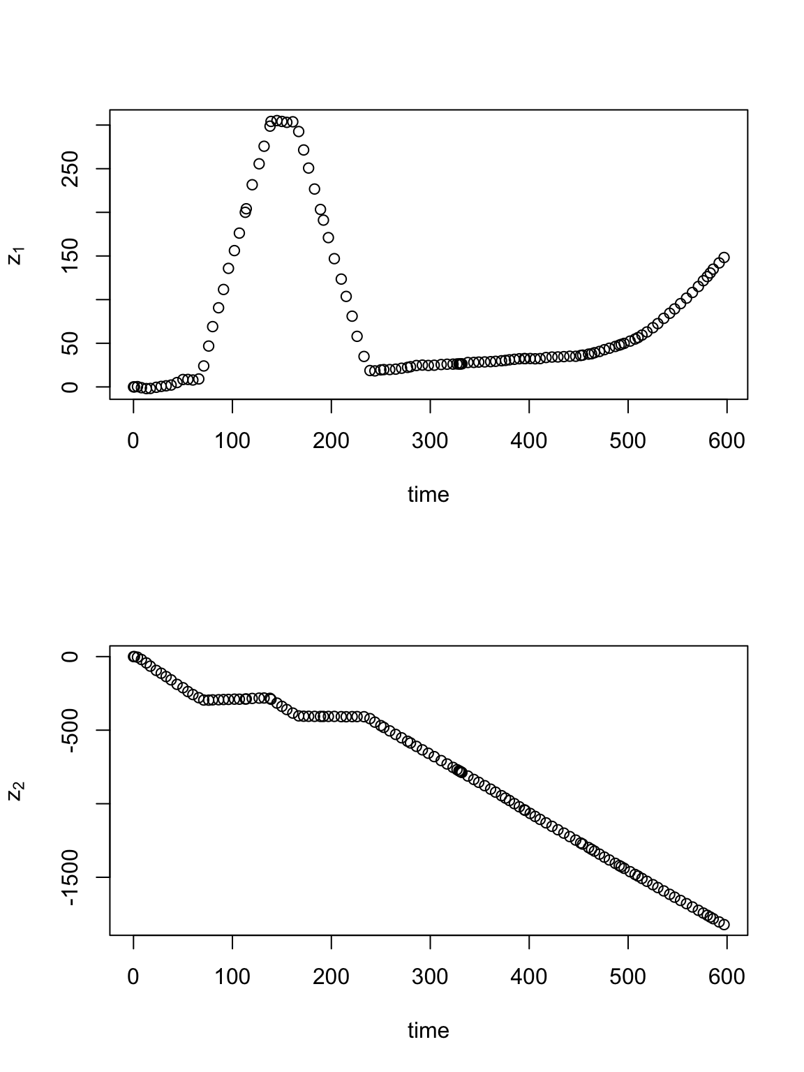
z <- cbind(df.traj$z1.obs, df.traj$z2.obs)
t.obs <- df.traj$t.obs
t <- seq(0, 660, by = 10)
K <- diag(1, length(t))[findInterval(unique(t.obs), t), ]
H <- matrix(1, length(t), length(t))
upperTriangle(H, diag = FALSE) <- 0
H <- H %*% H
KH <- K %*% H
KHpKH <- t(KH) %*% KH
dt <- c(1, diff(t))
n <- 2 * length(t)


m.draws <- 1000  #Number of MCMC samples to draw
samples <- as.data.frame(matrix(, m.draws + 1, 2))
colnames(samples) <- c("sigma2.z", "sigma2.alpha")
samples[1, ] <- c(2, 1)  #Starting values for sigma2.z, sigma2.alpha
samples.alpha1 <- matrix(, m.draws + 1, length(t))
samples.alpha2 <- matrix(, m.draws + 1, length(t))

# Hyperparameters for parameter models
q.alpha <- 2.01
r.alpha <- 1
q.z <- 2.01
r.z <- 1

set.seed(3909)
for (k in 1:m.draws) {

    sigma2.z <- samples[k, 1]
    sigma2.alpha <- samples[k, 2]
    C <- diag(dt)
    CI <- solve(C)

    # Sample alpha1 & alpha2
    A <- solve((1/sigma2.z) * KHpKH + 1/sigma2.alpha * CI)
    b1 <- (1/sigma2.z) * t(KH) %*% z[, 1]
    b2 <- (1/sigma2.z) * t(KH) %*% z[, 2]
    alpha1 <- mvrnorm(1, A %*% b1, A)
    alpha2 <- mvrnorm(1, A %*% b2, A)

    # Sample sigma2.alpha
    sigma2.alpha <- 1/rgamma(1, q.alpha + n/2, r.alpha + (t(alpha1) %*% CI %*%
        (alpha1) + t(alpha2) %*% CI %*% (alpha2))/2)

    # Sample sigma2.e
    sigma2.z <- 1/rgamma(1, q.z + n/2, r.z + (t(z[, 1] - KH %*% alpha1) %*%
        (z[, 1] - KH %*% alpha1) + t(z[, 2] - KH %*% alpha2) %*% (z[, 2] - KH %*%
        alpha2))/2)

    # Save
    samples[k + 1, ] <- c(sigma2.z, sigma2.alpha)
    samples.alpha1[k + 1, ] <- alpha1
    samples.alpha2[k + 1, ] <- alpha2
    # if(k%%100==0) print(k)
}


par(mfrow = c(2, 1))
plot(samples[, 1], typ = "l", xlab = "k", ylab = expression(sigma[z]^2))
plot(samples[, 2], typ = "l", xlab = "k", ylab = expression(sigma[alpha]^2))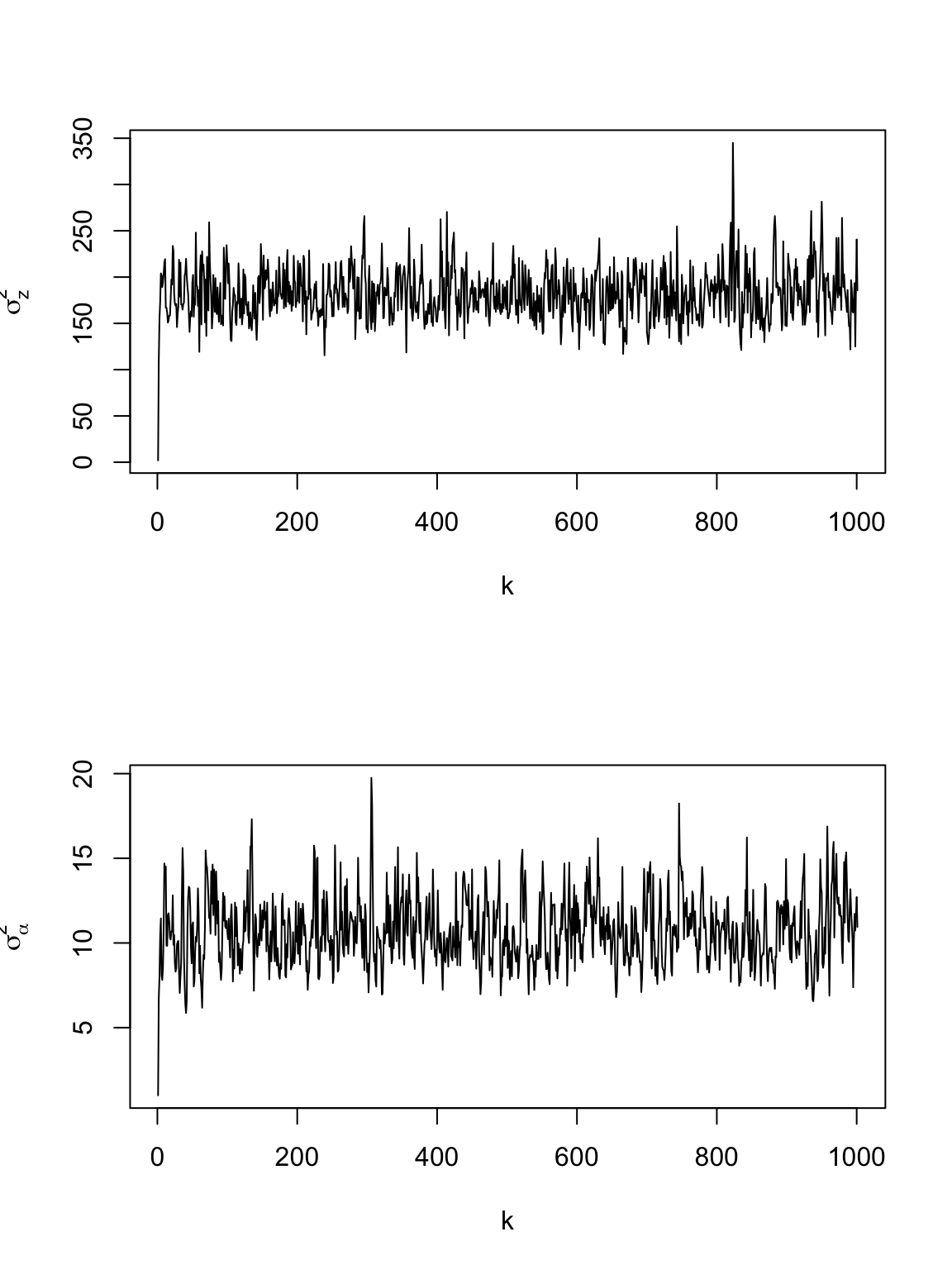
burn.in <- 100
y1.pred <- matrix(, m.draws - burn.in, length(t))
y2.pred <- matrix(, m.draws - burn.in, length(t))
for (k in burn.in:m.draws) {
    y1.pred[k - burn.in, ] <- H %*% samples.alpha1[k, ]
    y2.pred[k - burn.in, ] <- H %*% samples.alpha2[k, ]
}


# Plot time series of spatial location
par(mfrow = c(2, 1))
plot(df.traj$t.obs, df.traj$z1.obs, typ = "p", xlab = "time", ylab = expression(z[1]),
    xlim = c(0, 660))
points(t, colMeans(y1.pred), typ = "l", col = "red", lwd = 3)
lwr.CI <- apply(y1.pred, 2, FUN = quantile, prob = c(0.025))
upper.CI <- apply(y1.pred, 2, FUN = quantile, prob = c(0.975))
polygon(c(t, rev(t)), c(lwr.CI, rev(upper.CI)), col = rgb(0.5, 0.5, 0.5, 0.3),
    border = NA)

plot(df.traj$t.obs, df.traj$z2.obs, typ = "p", xlab = "time", ylab = expression(z[2]),
    xlim = c(0, 660), ylim = c(-2500, 0))
points(t, colMeans(y2.pred), typ = "l", col = "red", lwd = 3)
lwr.CI <- apply(y2.pred, 2, FUN = quantile, prob = c(0.025))
upper.CI <- apply(y2.pred, 2, FUN = quantile, prob = c(0.975))
polygon(c(t, rev(t)), c(lwr.CI, rev(upper.CI)), col = rgb(0.5, 0.5, 0.5, 0.3),
    border = NA)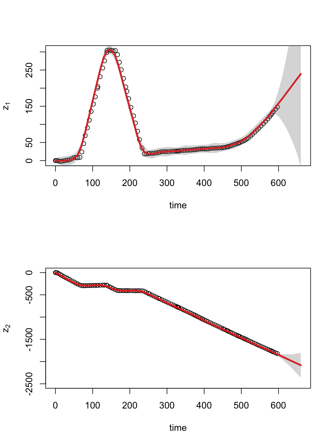
sf.s.pred.mmm.10min.ev <- spLines(cbind(colMeans(y1.pred) + df.traj$s1.obs[1],
    colMeans(y2.pred) + df.traj$s2.obs[1]), crs = crs(pt.traj))
lwr.CI.y1 <- apply(y1.pred, 2, FUN = quantile, prob = c(0.025))
lwr.CI.y2 <- apply(y2.pred, 2, FUN = quantile, prob = c(0.025))
upper.CI.y1 <- apply(y1.pred, 2, FUN = quantile, prob = c(0.975))
upper.CI.y2 <- apply(y2.pred, 2, FUN = quantile, prob = c(0.975))
sf.s.pred.mmm.10min.lci <- spLines(cbind(lwr.CI.y1 + df.traj$s1.obs[1], lwr.CI.y2 +
    df.traj$s2.obs[1]), crs = crs(pt.traj))
sf.s.pred.mmm.10min.uci <- spLines(cbind(upper.CI.y1 + df.traj$s1.obs[1], upper.CI.y2 +
    df.traj$s2.obs[2]), crs = crs(pt.traj))

par(mfrow = c(1, 1))
plot(pt.traj)
plot(sf.s.pred.mmm.10min.ev, lwd = 3, col = "red", add = TRUE)
plot(sf.s.pred.mmm.10min.lci, lwd = 3, col = "gold", lty = 2, add = TRUE)
plot(sf.s.pred.mmm.10min.uci, lwd = 3, col = "gold", lty = 2, add = TRUE)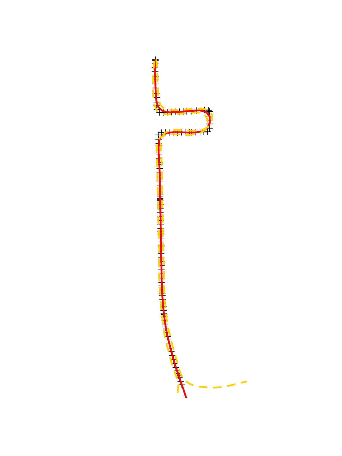
20.3 Summary
- Spatio-temporal modeling of trajectories (i.e., movement data) is an emerging area of research
- Model based vs. summary statistics
- Current and future research
- Inference from multiple trajectories (e.g., multiple people running the same marathon)
- Summarizing single trajectories
- Fitting models to “big data”
- Model selection
- Inclusion of predictor variables
- Influence of other moving objects (e.g., networks of moving animals)
- Constrained support of movement process