11 September 22
11.1 Announcements
- Assignment #3 is posted and due next week.
11.2 Extreme precipitation in Kansas
- What we will need to learn
- How to use R as a geographic information system
- New general tools from statistics
- Gaussian process
- Metropolis and Metropolis–Hastings algorithms
- Gibbs sampler
- How to use the hierarchical modeling framework to describe Kriging
- Hierarchical Bayesian model vs. “empirical” hierarchical model
- Specialized language used in spatial statistics (e.g., range, nugget, variogram)
11.3 Gibbs sampler
- History
- Stochastic Relaxation, Gibbs Distributions, and the Bayesian Restoration of Images (Geman and Geman 1984))
- Sampling-Based Approaches to Calculating Marginal Densities (Gelfand and Smith 1990)
- The gibbs sampler is responsible for the recent “Bayesian revolution”
- Gibbs sampler
- See pg. 169 in book.
- In many cases the distribution we want to sample from is multivariate
- If we can sample from the univariate full-conditional distribution for each random variable of a multivariate distribution, then we can use a Gibbs sampler to obtain dependent sample from the multivariate distribution
11.3.1 Gibbs sampler: simple example
\[\boldsymbol{\theta}\sim\text{N}\Bigg(\mathbf{0},\bigg[\begin{array}{cc} 1 & \rho\\ \rho\ & 1 \end{array}\bigg]\Bigg)\] where \(\boldsymbol{\theta}\equiv(\theta_{1},\theta_{2})'\). Suppose we didn’t know how to sample from the multivariate normal distribution, but we could obtain the conditional distributions \([\theta_{1}|\theta_{2}]\) and \([\theta_{2}|\theta_{1}]\) which are \[\theta_{1}|\theta_{2}\sim\text{N}(\rho\theta_{2},1-\rho^{2})\] \[\theta_{2}|\theta_{1}\sim\text{N}(\rho\theta_{1},1-\rho^{2})\,.\] It turns out that if we iteratively sample from \([\theta_{1}|\theta_{2}]\) and then \([\theta_{2}|\theta_{1}]\) (or the other way around) we will obtain samples from \([\boldsymbol{\theta}]\).
11.3.2 Gibbs sampler: Bayesian linear model example
- The model
- Distribution of the process: “\(\mathbf{y}\) given \(\boldsymbol{\beta}\) and \(\sigma_{\varepsilon}^{2}\)” \[\mathbf{y}|\boldsymbol{\beta},\sigma_{\varepsilon}^{2}\sim\text{N}(\mathbf{X}\boldsymbol{\beta},\sigma_{\varepsilon}^{2}\mathbf{I})\] This is also sometimes called the process model.
- Distribution of the parameters: \(\boldsymbol{\beta}\) and \(\sigma_{\varepsilon}^{2}\) \[\boldsymbol{\beta}\sim\text{N}(\mathbf{0},\sigma_{\beta}^{2}\mathbf{I})\] \[\sigma_{\varepsilon}^{2}\sim\text{inverse gamma}(q,r)\]
- Computations and statistical inference
- Using Bayes rule (Bayes 1763) we can obtain the joint posterior distribution
\[[\boldsymbol{\beta},\sigma_{\varepsilon}^{2}|\mathbf{y}]=\frac{[\mathbf{y}|\boldsymbol{\beta},\sigma_{\varepsilon}^{2}][\boldsymbol{\beta}][\sigma_{\varepsilon}^{2}]}{\int\int [\mathbf{y}|\boldsymbol{\beta},\sigma_{\varepsilon}^{2}][\boldsymbol{\beta}][\sigma_{\varepsilon}^{2}]d\boldsymbol{\beta}d\sigma_{\varepsilon}^{2}}\]
- Statistical inference about a paramters is obtained from the marginal posterior distributions \[[\boldsymbol{\beta}|\mathbf{y}]=\int[\boldsymbol{\beta},\sigma_{\varepsilon}^{2}|\mathbf{y}]d\sigma_{\varepsilon}^{2}\] \[[\sigma_{\varepsilon}^{2}|\mathbf{y}]=\int[\boldsymbol{\beta},\sigma_{\varepsilon}^{2}|\mathbf{y}]d\boldsymbol{\beta}\]
- In practice it is difficult to find closed-form solutions for the marginal posterior distributions, but easy to find closed-form solutions for the conditional posterior distribtuions.
- Full-conditional distribtuions: \(\boldsymbol{\beta}\) and \(\sigma_{\varepsilon}^{2}\) \[\boldsymbol{\beta}|\sigma_{\varepsilon}^{2},\mathbf{y}\sim\text{N}\bigg{(}\big{(}\mathbf{X}^{\prime}\mathbf{X}+\frac{1}{\sigma_{\beta}^{2}}\mathbf{I}\big{)}^{-1}\mathbf{X}^{\prime}\mathbf{y},\sigma_{\varepsilon}^{2}\big{(}\mathbf{X}^{\prime}\mathbf{X}+\frac{1}{\sigma_{\beta}^{2}}\mathbf{I}\big{)}^{-1}\bigg{)}\] \[\sigma_{\varepsilon}^{2}|\mathbf{\boldsymbol{\beta}},\mathbf{y}\sim\text{inverse gamma}\left(q+\frac{n}{2},(r+\frac{1}{2}(\mathbf{y}-\mathbf{X}\boldsymbol{\beta})^{'}(\mathbf{y}-\mathbf{X}\boldsymbol{\beta}))^-1\right)\]
- How do you find the full-conditional distributions?
- Gibbs sampler for the Bayesian linear model
- Write out on the whiteboard
- Using Bayes rule (Bayes 1763) we can obtain the joint posterior distribution
\[[\boldsymbol{\beta},\sigma_{\varepsilon}^{2}|\mathbf{y}]=\frac{[\mathbf{y}|\boldsymbol{\beta},\sigma_{\varepsilon}^{2}][\boldsymbol{\beta}][\sigma_{\varepsilon}^{2}]}{\int\int [\mathbf{y}|\boldsymbol{\beta},\sigma_{\varepsilon}^{2}][\boldsymbol{\beta}][\sigma_{\varepsilon}^{2}]d\boldsymbol{\beta}d\sigma_{\varepsilon}^{2}}\]
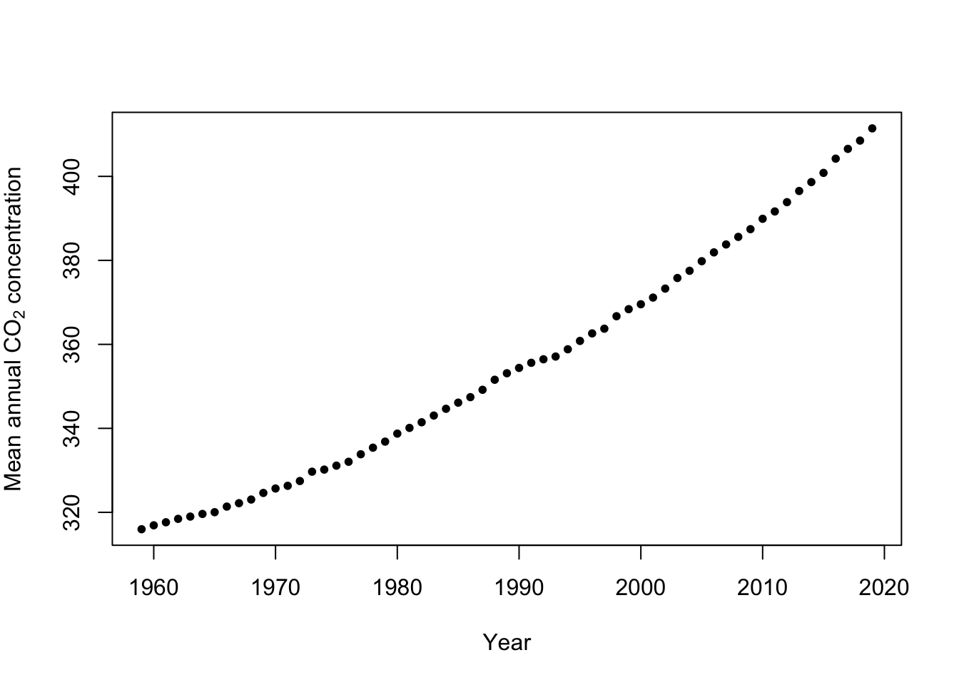
Example: Mauna Loa Observatory carbon dioxide data
url <- "ftp://aftp.cmdl.noaa.gov/products/trends/co2/co2_annmean_mlo.txt"
df <- read.table(url, header = FALSE)
colnames(df) <- c("year", "meanCO2", "unc")
plot(x = df$year, y = df$meanCO2, xlab = "Year", ylab = expression("Mean annual " *
    CO[2] * " concentration"), col = "black", pch = 20)
- Gibb sampler
# Preliminary steps
library(mvnfast)  # Required package to sample from multivariate normal distribution

y <- df$meanCO2  # Response variable
X <- model.matrix(~year, data = df)  # Design matrix
n <- length(y)  # Number of observations
p <- 2  # Dimensions of beta

m.draws <- 5000  #Number of MCMC samples to draw

samples <- as.data.frame(matrix(, m.draws, 3))  # Samples of the parameters we will save
colnames(samples) <- c(colnames(X), "sigma2")

sigma2.e <- 1  # Starting values for sigma2

sigma2.beta <- 10^9  #Prior variance for beta
q <- 2.01  #Inverse gamma prior with E() = 1/(r*(q-1)) and Var()= 1/(r^2*(q-1)^2*(q-2))
r <- 1


# MCMC algorithm
for (m in 1:m.draws) {
    # Sample beta from full-conditional distribution
    H <- solve(t(X) %*% X + diag(1/sigma2.beta, p))
    h <- t(X) %*% y
    beta <- t(mvnfast::rmvn(1, H %*% h, sigma2.e * H))

    # Sample sigma from full-conditional distribution
    q.temp <- q + n/2
    r.temp <- (1/r + t(y - X %*% beta) %*% (y - X %*% beta)/2)^-1
    sigma2.e <- 1/rgamma(1, q.temp, , r.temp)

    # Save samples of beta and sigma
    samples[m, ] <- c(beta, sigma2.e)
}

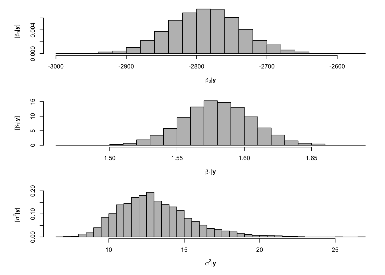
# Look a histograms of posterior distributions
par(mfrow = c(3, 1), mar = c(5, 6, 1, 1))
hist(samples[, 1], xlab = expression(beta[0] * "|" * bold(y)), ylab = expression("[" *
    beta[0] * "|" * bold(y) * "]"), freq = FALSE, col = "grey", main = "", breaks = 30)
hist(samples[, 2], xlab = expression(beta[1] * "|" * bold(y)), ylab = expression("[" *
    beta[1] * "|" * bold(y) * "]"), freq = FALSE, col = "grey", main = "", breaks = 30)
hist(samples[, 3], xlab = expression(sigma^2 * "|" * bold(y)), ylab = expression("[" *
    sigma^2 * "|" * bold(y) * "]"), freq = FALSE, col = "grey", main = "", breaks = 30)
## (Intercept) year ## -2787.515552 1.580116## X(Intercept) Xyear ## -2787.874923 1.580296
11.4 Metropolis algorithm
- Metropolis algorithm
- Suppose we know the analytical form of a function that is proportional to some density function but we don’t know how to sample from it.
- Example: \([\phi|y]\propto [y|\phi][\phi]\)
- The distribution we want to sample from is called the target distribution
- Obtain the analytical form of a function \(f(\cdot)\) that is proportional to the target distribution.
- Let \(\phi^{*}\) be a single draw from a proposal distribution \([\phi^{*}]\) that is symmetric and easy to sample from. For convenience, make sure the proposal has the same support as the target distribution
- Algorithm
- set an initial value for \(\phi^{(1)}\)
- while k < m do
- obtain \(\phi^{*}\) by sampling from \([\phi^{*}]\)
- calculate \(R = \text{min}\big(1,\frac{f(\phi^{*})}{f(\phi^{(k)})}\big)\)
- set \(\phi^{(k+1)}\) to \(\phi^{*}\) with probability \(R\) else \(\phi^{(k)}\)
- end while
- Suppose we know the analytical form of a function that is proportional to some density function but we don’t know how to sample from it.
- Efficiency and the proposal distribution
- The Metropolis algorithm produces dependent samples from the target distribution.
- Since we can pick any symmetric proposal distribution, we should pick one that results in a higher effective sample size to increase efficiency.
We should also keep track of the acceptance rate (i.e., when we keep the proposed value \(\phi^{*}\).
Example (Using normal proposal)
library(latex2exp)

# Let's sample from a beta distribution
m <- 1000 # Number of samples
set.seed(2030)
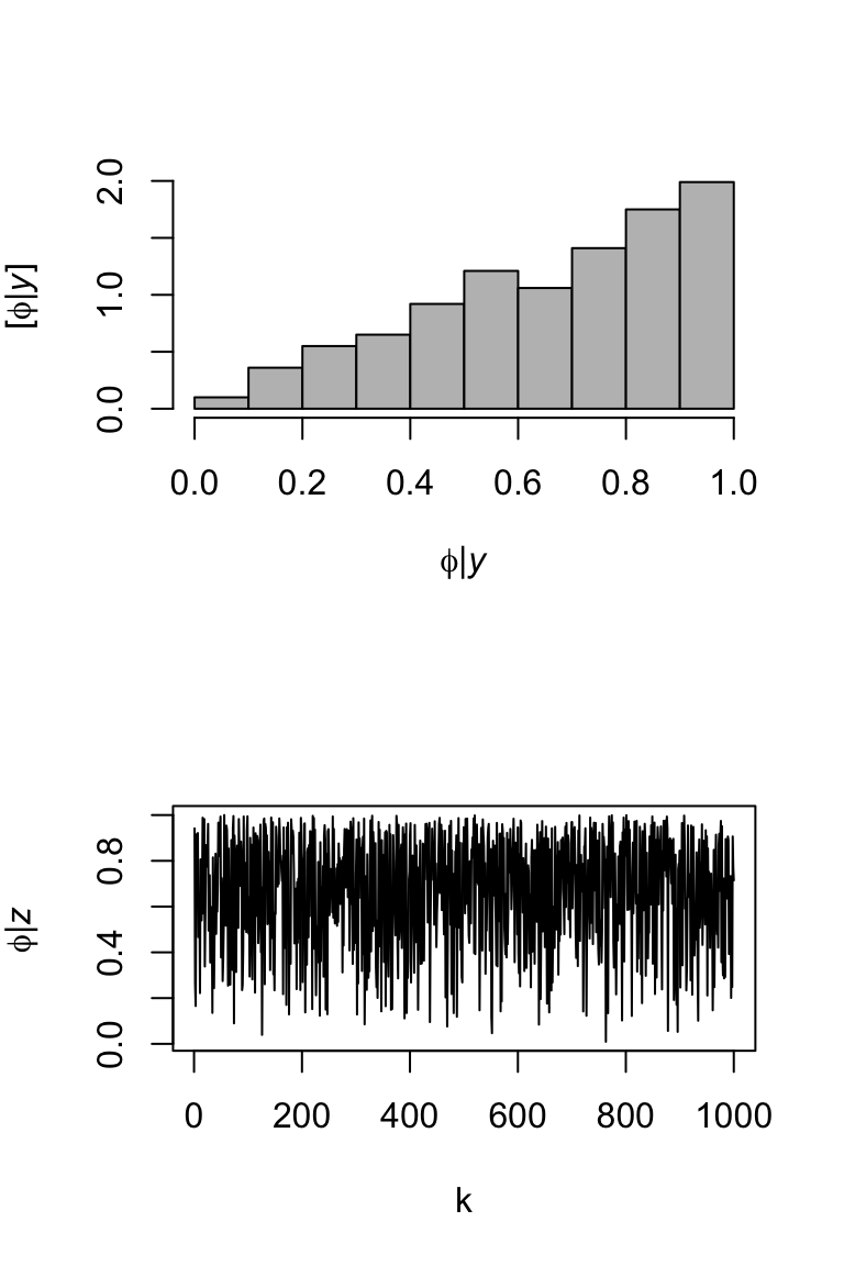
phi.iid <- rbeta(m,2,1)

library(coda)
effectiveSize(phi.iid)
## var1 ## 1000par(mfrow=c(2,1)) hist(phi.iid,col="grey",freq=FALSE,main="", xlab= TeX('$\\phi | \\mathit{y}$'), ylab = TeX('$\\lbrack\\phi | \\mathit{y}\\rbrack$')) plot(phi.iid,typ="l",xlab="k",ylab= TeX('$\\phi | \\mathit{z}$'))
# Now assume we couldn't use rbeta()
phi <- matrix(,m+1,1) # (m+1) x 1 vector to save samples of x in
phi[1,] <- 0.5 # Starting value

set.seed(1603)
for(i in 1:m){
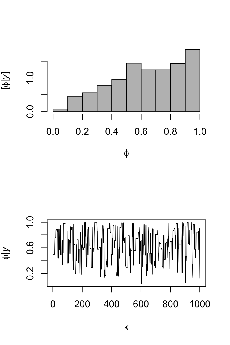
  phi.star <- rnorm(1,0.5,1) # Normal proposal distribution
  if((phi.star > 0) & (phi.star < 1)){
R <- min(1,(dbinom(1,1,phi.star)*dbeta(phi.star,1,1))/(dbinom(1,1,phi[i,1])*dbeta(phi[i,1],1,1)))
}else{R <- 0}
  if(R > runif(1)){phi[i+1,] <- phi.star}else{phi[i+1,] <- phi[i,1]} #Retain phi.star with probability R
}

effectiveSize(phi)
## var1 ## 128.858par(mfrow=c(2,1)) hist(phi,col="grey",freq=FALSE,main="", xlab= TeX('$\\phi$'), ylab = TeX('$\\lbrack\\phi | \\mathit{y}\\rbrack$')) plot(phi,typ="l",xlab="k",ylab= TeX('$\\phi | \\mathit{y}$'))
11.5 Metropolis-Hastings algorithm
- Understanding the Metropolis-Hastings algorithm (Chib and Greenberg 1995)
- Similar to the Metropolis algorithm, but the proposal distribution does not have to be symmetric.
- Modifications to the Metropolis algorithm
- \(R=\text{min}\big(1,\frac{f(\phi^{*})}{f(\phi^{(k)})}\times\frac{[\phi^{(k)}]}{[\phi^{*}]}\big)\) where \([\phi^{(k)}]\) and \([\phi^{*}]\) is the pdf/pmf of the proposal distribution evaluated at \(\phi^{(k)}\) and \(\phi^{*}\) respectively