5 September 1
5.1 Announcements
- Office hours 9:30 - 10:30 today or by appointment
- Lots of good questions are being asked and answered!
- Poll
- Questions about assignment 2?
5.2 Bayesian hierarchical models
- Review of the Bayesian hierarchical modeling framework
\[\text{Data model:} \;\;[\mathbf{z}|\mathbf{y},\boldsymbol{\theta}_{D}]\] \[\text{Process model:} \;\;[\mathbf{y}|\boldsymbol{\theta}_{P}]\] \[\text{Parameter model:} \;\;[\boldsymbol{\theta}]\]
5.2.1 Motivating data example
- Whooping cranes
Data set
url <- "https://www.dropbox.com/s/ihs3as87oaxvmhq/Butler%20et%20al.%20Table%201.csv?dl=1"
df1 <- read.csv(url)

plot(df1$Winter, df1$N, xlab = "Year", ylab = "Population count (z)", xlim = c(1940,
    2020), ylim = c(0, 300), typ = "b", cex = 0.8, pch = 20, col = rgb(0.7,
    0.7, 0.7, 0.9))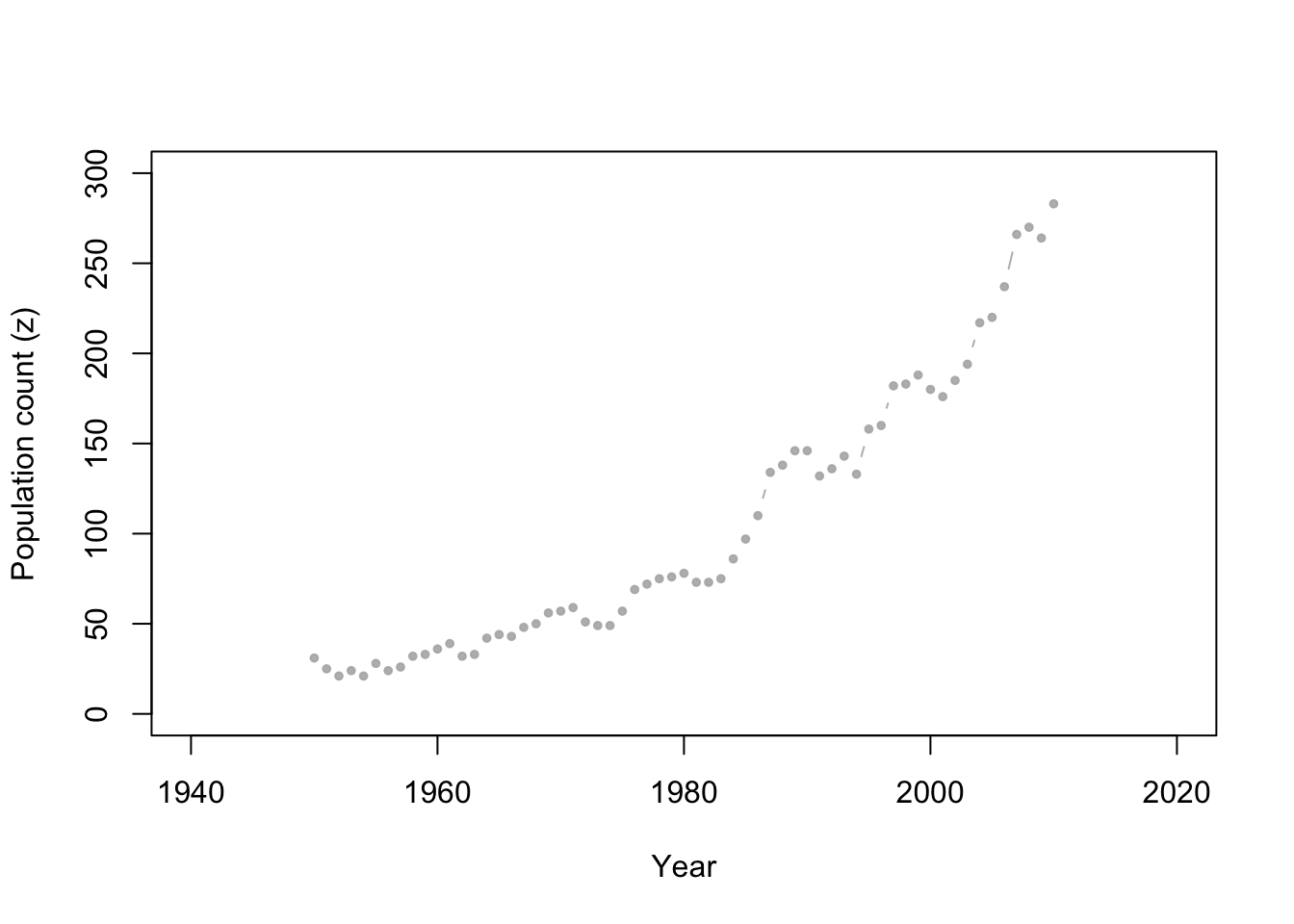
Write out a Bayesian hierarchical model for the whooping crane data
5.2.2 Simulating data from the prior predictive distribution
- The prior predictive distribution is capable of providing predictions/forecasts without the use of any data
- Other fields call this “simulation modeling” or a “sensitivity analysis”
- It is basically data free statistics (i.e., prediction, forecasts, and inference is 100% assumption driven)
- Used as a form of model (assumption) checking in Bayesian statistics
- Super easy to do and helps us “prototype” our statistical model before we put in any more work
- Live demonstration in R for the whooping crane data example
- Warning about using the data twice
5.2.3 Model fitting
- Class discussion
- Markov chain Monte Carlo
- Algorithm 4.2 (see pg. 169 in Wikle et al. 2019)
- Next time in class
- Rejection sampling and Approximate Bayesian computation
- Live demonstration in R for the whooping crane data example
# Download and view data
url <- "https://www.dropbox.com/s/ihs3as87oaxvmhq/Butler%20et%20al.%20Table%201.csv?dl=1"
df1 <- read.csv(url)
head(df1)
## Winter N
## 1 1950 31
## 2 1951 25
## 3 1952 21
## 4 1953 24
## 5 1954 21
## 6 1955 28# Required functions
calc.lambda <- function(t, t0, gamma, lambda0) {
lambda0 * exp(gamma * (t - t0))
}
rdunif <- function(n, min, max) {
sample(min:max, size = n, replace = TRUE)
}
# Algorithm settings
K.tries <- 10^6 # Number of simulated data sets to make
diff <- matrix(, K.tries, 1) # Vector to save the measure of discrepancy between simulated data and real data
error <- 1000 # Allowable difference between simulated data and real data
# Known random variables and parameters
t0 <- 1949
t <- df1$Winter
z <- df1$N
n <- length(z)
# Unkown random variables and parameters
posterior.samp.parameters <- matrix(, K.tries, 3) # Matrix to samples of save unknown parameters
colnames(posterior.samp.parameters) <- c("gamma", "lambda0", "p")
y <- matrix(, K.tries, n) # Matrix to samples of save unknown number of whooping cranes
for (k in 1:K.tries) {
# Simulate from the prior predictive distribution
gamma.try <- runif(1, 0, 0.1) # Parameter model
lambda0.try <- rdunif(1, 2, 50) # Parameter model
lambda.try <- calc.lambda(t = t, t0 = t0, gamma = gamma.try, lambda0 = lambda0.try) # Mathematical equation for process model
y.try <- rpois(n, lambda.try) # Process model
p.try <- runif(1, 0, 1) # Prior or data model
z.try <- rbinom(n, y.try, p.try) # Data model
# Record difference between draw of z from prior predictive distribution and
# observed data
diff[k, ] <- sum(abs(z - z.try))
# Save unkown random variables and parameters
y[k, ] <- y.try
posterior.samp.parameters[k, ] <- c(gamma.try, lambda0.try, p.try)
}
# Calculate acceptance rate
length(which(diff < error))/K.tries## [1] 0.015703# Plot approximate posterior distribution of parameters
library(latex2exp)
hist(posterior.samp.parameters[which(diff < error), 1], col = "grey", freq = FALSE,
xlim = c(0, 0.1), main = "", xlab = TeX("$\\gamma | \\mathbf{z}$"), ylab = TeX("$\\lbrack\\gamma | \\mathbf{z}\\rbrack$"))
curve(dunif(x, 0, 0.1), col = "deepskyblue", lwd = 3, add = TRUE)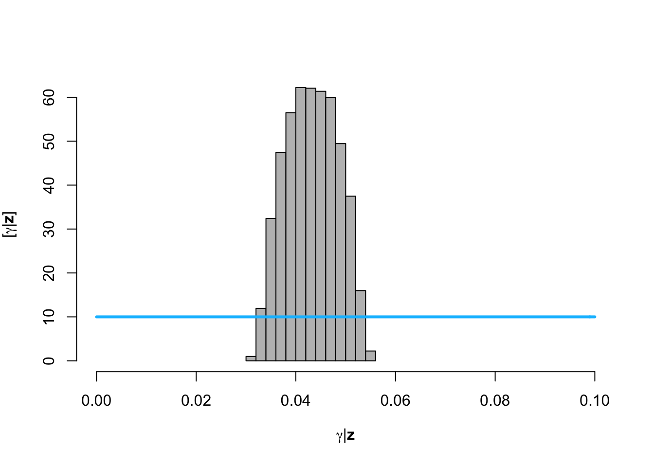
hist(posterior.samp.parameters[which(diff < error), 2], col = "grey", freq = FALSE,
    xlim = c(2, 50), main = "", breaks = seq(2, 50, by = 1), xlab = TeX("$\\lambda_0  | \\mathbf{z}$"),
    ylab = TeX("$\\lbrack\\lambda_0  | \\mathbf{z}\\rbrack$"))
curve(dunif(x, 2, 50), col = "deepskyblue", lwd = 3, add = TRUE)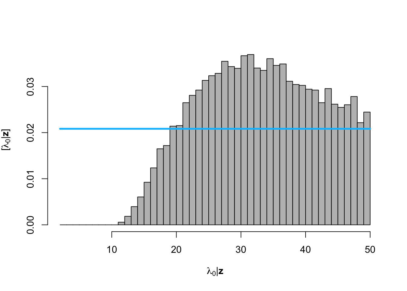
hist(posterior.samp.parameters[which(diff < error), 3], col = "grey", freq = FALSE,
    xlim = c(0, 1), main = "", xlab = TeX("$\\p  | \\mathbf{z}$"), ylab = TeX("$\\lbrack\\p  | \\mathbf{z}\\rbrack$"))
curve(dunif(x, 0, 1), col = "deepskyblue", lwd = 3, add = TRUE)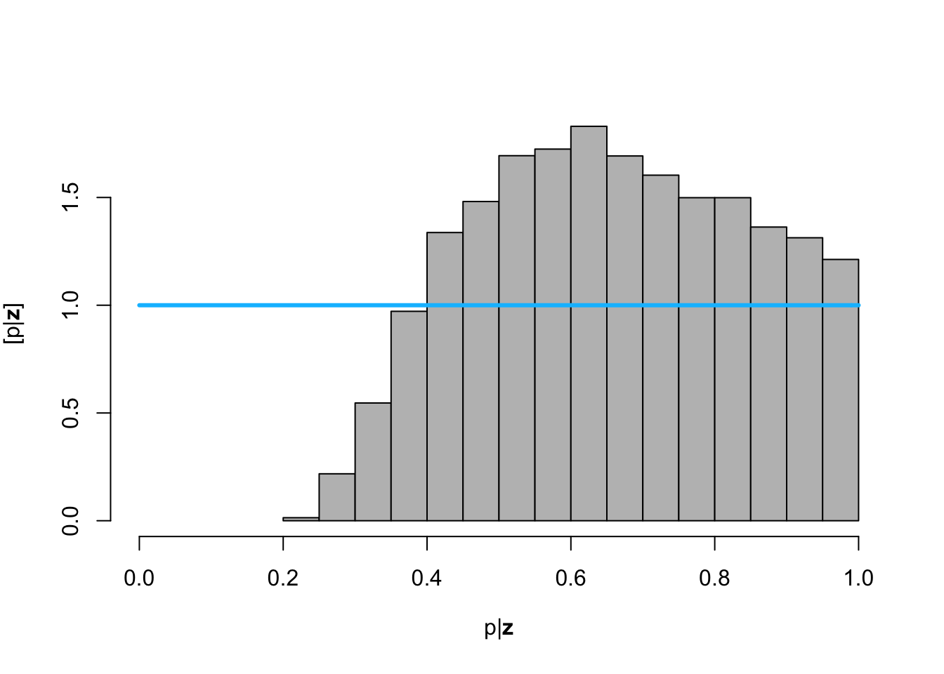
# Plot data (z) and approximate posterior distribution of y
plot(df1$Winter, df1$N, xlab = "Year", ylab = "True population size (y)", xlim = c(1940,
    2010), ylim = c(0, 1000), typ = "b", cex = 0.8, pch = 20, col = rgb(0.7,
    0.7, 0.7, 0.9))
e.y <- colMeans(y[which(diff < error), ])
points(df1$Winter, e.y, typ = "l", lwd = 2)
lwr.CI <- apply(y[which(diff < error), ], 2, FUN = quantile, prob = c(0.025))
upper.CI <- apply(y[which(diff < error), ], 2, FUN = quantile, prob = c(0.975))
polygon(c(df1$Winter, rev(df1$Winter)), c(lwr.CI, rev(upper.CI)), col = rgb(0.5,
    0.5, 0.5, 0.3), border = NA)
legend(x = 1940, y = 1000, cex = 1.3, legend = c(expression("E(" * y[pred] *
    "|" * z * ")"), "95% CI"), bty = "n", lty = 1, lwd = 2, col = c("black",
    rgb(0.5, 0.5, 0.5, 0.5)))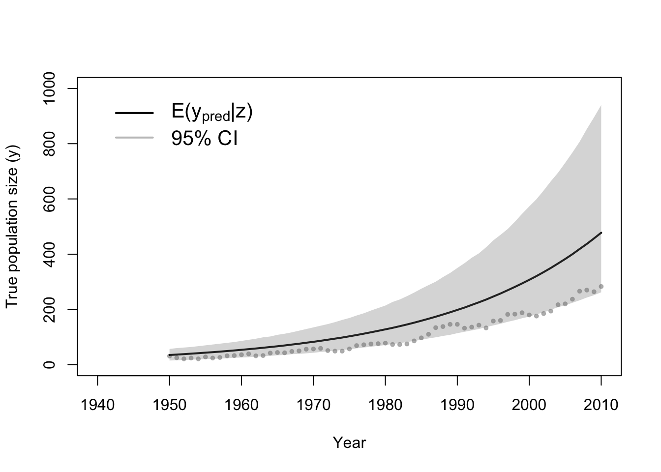
5.3 Summary and comments
- Bayesian hierarchical modeling framework is incredibly flexible
- Motivated by a data set or practical problem, you can build your own “custom” statistical models
- You can always “turn the Bayesian crank” for whatever model you develop (with some warnings of course!)
- Practice the process of model specification (what we did today in class) at home on a different data set