Chapter 20 Survival Analysis
20.1 What is survival data?
Time-to-event data that consists of a distinct start time and end time. These data are common in the medical field.
Examples from cancer:
- Time from surgery to death
- Time from start of treatment to progression
- Time from response to recurrence
20.1.1 Examples from other fields
Time-to-event data is common in many fields including, but not limited to:
- Crime: Time from release to criminal recidivism
- Marketing: Customer retention
- Engineering: Time to machine malfunction
- Finance: Time to loan default
- Management: Time to employee resignation/termination
20.2 Questions of interest
The two most common questions I encounter related to survival analysis are:
- What is the probability of survival to a certain point in time?
- What is the average survival time?
20.3 What is censoring?
In survival analysis, it is common for the exact event time to be unknown, or unobserved, which is called censoring. A subject may be censored due to:
- Loss to follow-up
- Withdrawal from study
- No event by end of fixed study period
Specifically these are examples of right censoring. Other common types of censoring include:
- Left (you do not observed the beginning)
- Interval (individual is loss during the study)
20.3.1 Censored survival data
When the exact event time is unknown then some patients are censored, and survival analysis methods are required.
We can incorporate censored data using survival analysis techniques
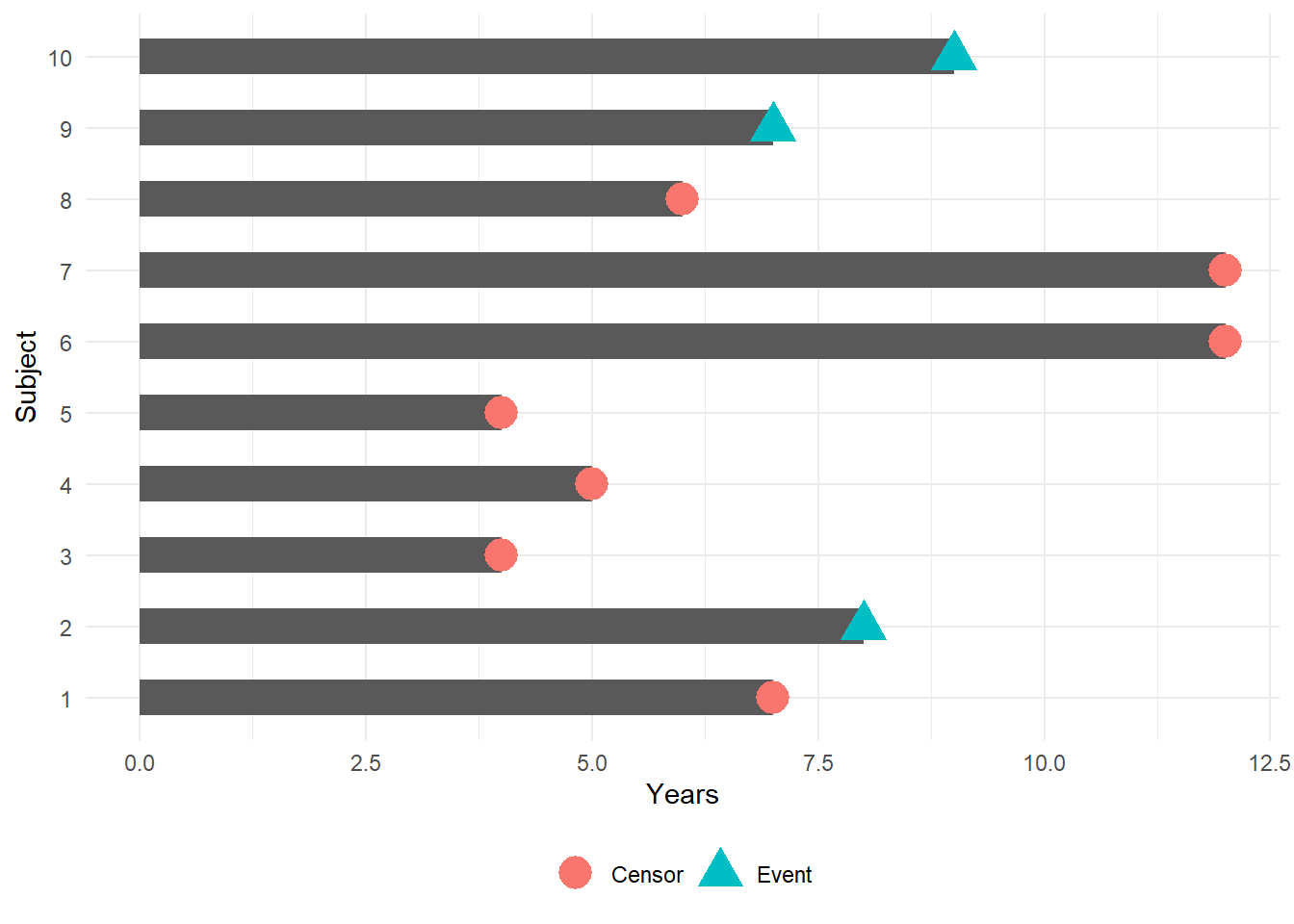
Toy example of a Kaplan-Meier curve for this simple data (details to follow):
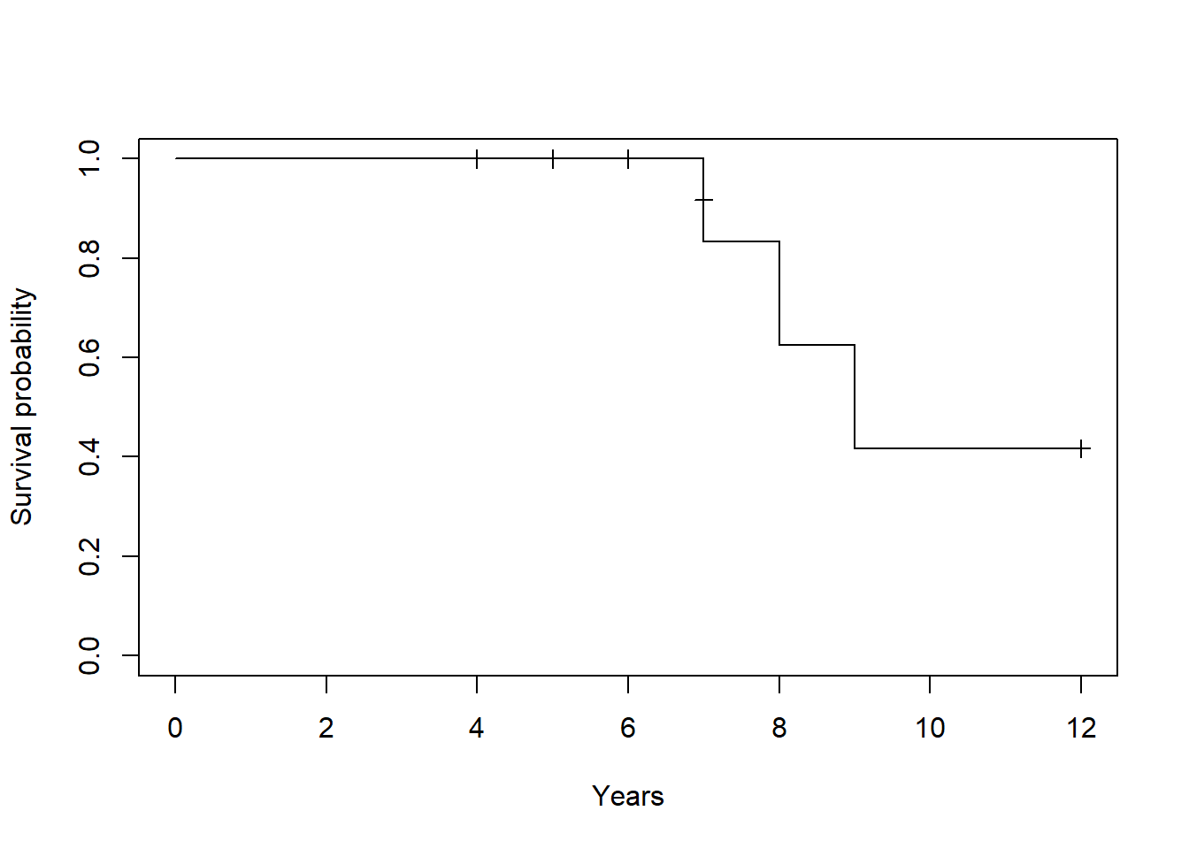
- Horizontal lines represent survival duration for the interval
- An interval is terminated by an event
- The height of vertical lines show the change in cumulative probability
- Censored observations, indicated by tick marks, reduces the cumulative survival between intervals
20.4 Danger of ignoring censoring
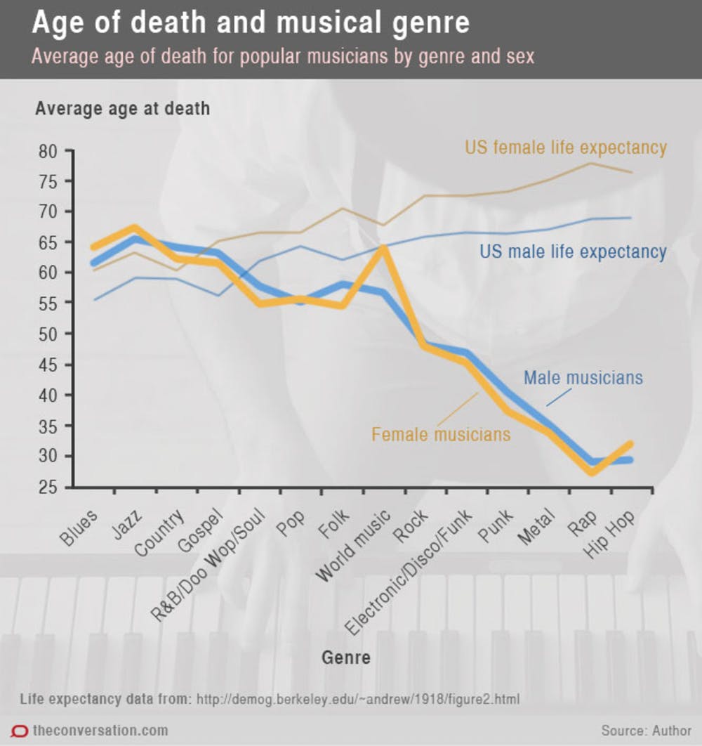
Case study: musicians and mortality
Conclusion: Musical genre is associated with early death among musicians.
Problem: this graph does not account for the right-censored nature of the data.
20.5 Components of survival data
For subject \(i\):
Event time \(T_i\)
Censoring time \(C_i\)
Event indicator \(\delta_i\):
- 1 if event observed (i.e. \(T_i \leq C_i\))
- 0 if censored (i.e. \(T_i > C_i\))
Observed time \(Y_i = \min(T_i, C_i)\)
20.6 Data example
20.6.1 Research question of interest
Organ Transplantation is limited by the supply of cadaveric and living donors.
Unfortunately, many people die while waiting on the list.
What types of characteristics lead to an increase or decrease likelihood of dying on the waiting list?
20.6.2 Data structure
- 815 of people on the waiting list
- Outcome: Death
- Predictors: age, sex, Blood type, year added to list
##   age sex abo year futime    event
## 1  47   m   B 1994   1197    death
## 2  55   m   A 1991     28      ltx
## 3  52   m   B 1996     85      ltx
## 4  40   f   O 1995    231      ltx
## 5  70   m   O 1996   1271 censored
## 6  66   f   O 1996     58      ltx
20.6.3 Variables:
- “futime”: the observed time \(Y_i = min(T_i, C_i)\)
- “event”: the event factor variable can take on censored, death, liver transplant, or withdraw
- “abo”: blood type A, B, AB, or O
- sex: Male or Female
- age: age at addition to the waiting list
20.6.4 Preparing data for analysis
Event indicator
Most functions used in survival analysis will also require a binary indicator of event that is:
- 0 for no event
- 1 for event
Currently our data example contains a factor variable indicating whether the patient has died or if they have received a liver transplant, been withdrawn, or are censored.
20.7 Analyzing survival data
20.7.1 Questions of interest
Recall the questions of interest:
- What is the probability of surviving to a certain point in time?
- What is the average survival time?
20.7.2 Creating survival objects
The Kaplan-Meier method is the most common way to estimate survival times and probabilities. It is a non-parametric approach that results in a step function, where there is a step down each time an event occurs.
- The
Survfunction from thesurvivalpackage creates a survival object for use as the response in a model formula. - There will be one entry for each subject that is the survival time, which is followed by a
+if the subject was censored.
Let’s look at the first 10 observations:
## [1] 1197 28+ 85+ 231+ 1271+ 58+ 392+ 30+ 12+ 139+20.7.3 Estimating survival curves with the Kaplan-Meier method
- The
survival::survfitfunction creates survival curves based on a formula. Let’s generate the overall survival curve for the entire cohort, assign it to objectf1, and look at thenamesof that object:
##  [1] "n"         "time"      "n.risk"    "n.event"   "n.censor"  "surv"
##  [7] "std.err"   "cumhaz"    "std.chaz"  "type"      "logse"     "conf.int"
## [13] "conf.type" "lower"     "upper"     "call"
Some key components of this survfit object that will be used to create survival curves include:
time, which contains the start and endpoints of each time intervalsurv, which contains the survival probability corresponding to eachtime
20.7.4 Kaplan-Meier plot - base R
Now we plot the survfit object in base R to get the Kaplan-Meier plot:
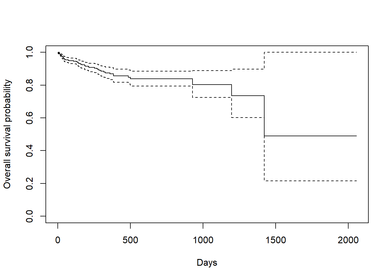
- The default plot in base
Rshows the step function (solid line) with associated confidence intervals (dotted lines). Note that the tick marks for censored patients are not shown by default, but could be added usingmark.time = TRUE
20.7.5 Estimating survival time
One quantity often of interest in a survival analysis is the probability of surviving a certain number \((x)\) of years.
For example, to estimate the probability of surviving to 5 years, use summary with the times argument:
## Call: survfit(formula = Surv(transplant$futime, transplant$delta) ~
##     1, data = transplant)
##
##  time n.risk n.event survival std.err lower 95% CI upper 95% CI
##  1825      2      66     0.49   0.206        0.215            1
We find that the 5-year probability of survival in this study is 49%. The associated lower and upper bounds of the 95% confidence interval are also displayed.
20.7.6 Survival time is often estimated incorrectly
What happens if you use a “naive” estimate?
66 of the 815 patients died by 5 years so:
\[\Big(1 - \frac{66}{815}\Big) \times 100 = 92\%\]
You get an incorrect estimate of the 5-year probability of survival when you ignore the fact that 747 patients were censored before 5 years.
Recall the correct estimate of the 5-year probability of survival was 49%.
20.7.7 Estimating median survival time
Another quantity often of interest in a survival analysis is the average survival time, which we quantify using the median (survival times are not expected to be normally distributed so the mean is not an appropriate summary).
We can obtain this directly from our survfit object:
## Call: survfit(formula = survival::Surv(futime, delta) ~ 1, data = transplant)
##
##        n events median 0.95LCL 0.95UCL
## [1,] 815 66 1422 1422 NAWe see the median survival time is 3.9 years. The lower and upper bounds of the 95% confidence interval are also displayed.
20.7.8 Median survival is often estimated incorrectly
What happens if you use a “naive” estimate?
Summarize the median survival time among the 66 patients who died:
## [1] 65.5You get an incorrect estimate of median survival time of 0.2 years when you ignore the fact that censored patients also contribute follow-up time.
Recall the correct estimate of median survival time is 3.9 years.
20.8 Comparing survival times between groups
20.8.1 Questions of interest with respect to between-group differences
Is there a difference in survival probability between groups?
From our example: does the probability of survival differ according to gender among liver transplant patients?
20.8.2 Kaplan-Meier plot by group
We can add a covariate to the right-hand side of the survival::survfit object to obtain a stratified Kaplan-Meier plot.
Let’s also look at some other customization we can do with survminer::ggsurvplot.
survminer::ggsurvplot(
    fit = survival::survfit(survival::Surv(futime, delta) ~ abo, data = transplant),
    xlab = "Days",
    ylab = "Overall survival probability",
    legend.title = "Blood Type",
    legend.labs = c("A", "B", "AB","O"),
    break.x.by = 100,
    censor = FALSE,
    risk.table = TRUE,
    risk.table.y.text = FALSE)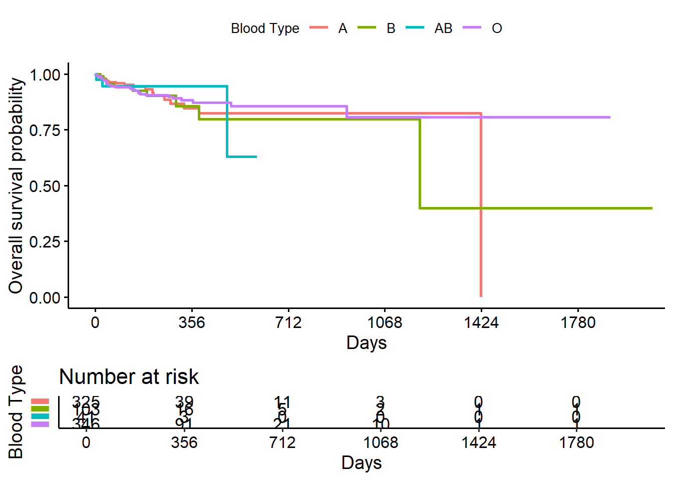
- Blood type B patients have the lowest overall survival probability.
- The risk table below the plot shows us the number of patients at risk at certain time points, which can give an idea of how much information is being used to calculate the estimates at each time
- Male patients have the lowest overall survival probability.
20.9 \(x\)-year survival probability by group
As before, we can get an estimate of, for example, 1-year survival by using summary with the times argument in our survival::survfit object:
## Call: survfit(formula = Surv(futime, delta) ~ sex, data = transplant)
##
##                 sex=m
##         time       n.risk      n.event     survival      std.err lower 95% CI
##     365.0000      82.0000      37.0000       0.8641       0.0244       0.8175
## upper 95% CI
##       0.9134
##
##                 sex=f
##         time       n.risk      n.event     survival      std.err lower 95% CI
##     365.0000      59.0000      22.0000       0.8763       0.0276       0.8238
## upper 95% CI
##       0.9322
20.10 Log-rank test for between-group significance test
- We can conduct between-group significance tests using a log-rank test.
- The log-rank test equally weights observations over the entire follow-up time and is the most common way to compare survival times between groups.
- There are versions that more heavily weight the early or late follow-up that could be more appropriate depending on the research question.
We get the log-rank p-value using the survival::survdiff function:
## Call:
## survival::survdiff(formula = Surv(futime, delta) ~ sex, data = transplant)
##
##         N Observed Expected (O-E)^2/E (O-E)^2/V
## sex=m 447       42     36.4     0.861      1.93
## sex=f 368       24     29.6     1.059      1.93
##
##  Chisq= 1.9  on 1 degrees of freedom, p= 0.2
And we see that the p-value is .2, indicating no significant difference in overall survival according to gender.
20.11 The Cox regression model
We may want to quantify an effect size for a single variable, or include more than one variable into a regression model to account for the effects of multiple variables.
The Cox regression model is a semi-parametric model that can be used to fit univariable and multivariable regression models that have survival outcomes.
Some key assumptions of the model:
- non-informative censoring
- proportional hazards
20.11.1 Cox regression example using a single covariate
We can fit regression models for survival data using the survival::coxph function, which takes a survival::Surv object on the left hand side and has standard syntax for regression formulas in R on the right hand side.
We can see a tidy version of the output using the tidy function from the broom package:
## # A tibble: 3 × 5
##   term          estimate std.error statistic p.value
##   <chr>            <dbl>     <dbl>     <dbl>   <dbl>
## 1 factor(abo)B    0.183      0.386    0.474    0.636
## 2 factor(abo)AB   0.195      0.618    0.316    0.752
## 3 factor(abo)O   -0.0110     0.284   -0.0388   0.969
20.11.2 Hazard ratios
The quantity of interest from a Cox regression model is a hazard ratio (HR).
If you have a regression parameter \(\beta\) (from column estimate in our survival::coxph) then HR = \(\exp(\beta)\).
For example, from our example we obtain the regression parameter \(\beta_1=0.195\) for AB vs B blood type, so we have HR = \(\exp(\beta_1)=1.21\).
A HR < 1 indicates reduced hazard of death whereas a HR > 1 indicates an increased hazard of death.
So we would say that a person with AB blood type has 1.21 times increased hazard of death as compared to a person with A blood type.
20.12 Summary
- Time-to-event data is common
- Survival analysis techniques are required to account for censored data
- The
survivalpackage provides tools for survival analysis, including theSurvandsurvfitfunctions - The
survminerpackage allows for customization of Kaplan-Meier plots based onggplot2 - Between-group comparisons can be made with the log-rank test using
survival::survdiff - Multivariate Cox regression analysis can be accomplished using
survival::coxph
20.13 Empoyee Attrition Example
# First let's import the data
q = read.csv('turnover2.csv', header = TRUE, sep = ",", na.strings = c("",NA))
Our case uses data of 1785 employees.
20.13.1 Variables:
\(exp\) - length of employment in the company
\(event\) - event (1 - terminated, 0 - currently employed)
\(branch\) - branch
\(pipeline\) - source of recruitment
Please note that the data is already prepared for survival analysis. Moreover, length of employment is counted in months up to two decimal places, according to the following formula: (date fire - date hire) / (365.25 / 12).
20.13.2 Cox Model
| Dependent variable: | |
| exp | |
| branchfirst | -0.089 (0.164) |
| branchfourth | -0.529c (0.176) |
| branchsecond | -0.424c (0.164) |
| branchthird | -0.466b (0.210) |
| pipelineea | -0.214 (0.267) |
| pipelinejs | 0.503b (0.201) |
| pipelineref | 0.322 (0.214) |
| pipelinesm | 0.361 (0.258) |
| Observations | 1,785 |
| R2 | 0.037 |
| Max. Possible R2 | 1.000 |
| Log Likelihood | -6,767.031 |
| Wald Test | 63.260c (df = 8) |
| LR Test | 67.275c (df = 8) |
| Score (Logrank) Test | 64.850c (df = 8) |
| Note: | p<0.1; p<0.05; p<0.01 |
20.14 Accelerated failure-time models
20.14.1 survreg(formula, dist=‘weibull’)
An accelerated failure-time (AFT) model is a parametric model with covariates and failure times following the survival function of the form \(S(x|Z) = S_0 (x exp[\theta Z])\), where \(S_0\) is a function for the baseline survival rate. The term \(exp[\theta Z]\) is called the acceleration factor.
The AFT model uses covariates to place individuals on different time scales { note the scaling by the covariates in \(S(t|Z)\) via \(exp[\theta Z]\). The AFT model can be rewritten in a log-linear form, where the log of failure time (call this logX) is linearly related to the mean \(\mu\), the acceleration factor, and an error term \(\sigma W\): \[log X = \theta'Z+\sigma W\]
20.14.2 Different AFT Models
There are several AFT models depending on the assumption about the distribution of the error \(W\).
| Distribution | df | Included in Survival |
|---|---|---|
| Exponential | 1 | yes |
| Weibull | 2 | yes |
| lognormal | 2 | yes |
| log logistic | 2 | yes |
| generalized gamma | 3 | no |
20.14.3 Weibull
The Weibull distribution has a survival function equal to \[S(t)=exp(-(\lambda t)^\rho)\]
and a hazard function equal to \[\Lambda(t)=\rho \lambda(\lambda t)^{\rho-1}\]
where \(\lambda>0\) and \(\rho>0\). A special case of the Weibul functions is the exponential distribution when \(\rho=1\).
If \(\rho > 1\), then the risk increases over time.
If \(\rho < 1\), then the risk decreases over time.
20.14.4 Weibul Model in R
The survival package allows us to estimate all of these models. We will use the same model with a small change to estimate a Weibul AFT model.
20.14.5 Weibul Model in R
| exp | ||
| Weibull | exponential | |
| (1) | (2) | |
| branchfirst | 0.142 (0.147) | 0.119 (0.164) |
| branchfourth | 0.494*** (0.157) | 0.524*** (0.176) |
| branchsecond | 0.433*** (0.146) | 0.441*** (0.163) |
| branchthird | 0.434** (0.189) | 0.469** (0.210) |
| pipelineea | 0.228 (0.239) | 0.239 (0.267) |
| pipelinejs | -0.529*** (0.180) | -0.537*** (0.200) |
| pipelineref | -0.383** (0.192) | -0.372* (0.213) |
| pipelinesm | -0.376 (0.232) | -0.386 (0.258) |
| Constant | 1.831*** (0.220) | 1.860*** (0.245) |
| N | 1,785 | 1,785 |
| Log Likelihood | -2,712.426 | -2,721.241 |
| chi2 (df = 8) | 74.713*** | 69.134*** |
| Notes: | ***Significant at the 1 percent level. | |
| **Significant at the 5 percent level. | ||
| *Significant at the 10 percent level. | ||
20.14.6 Do we need accelerated time?
The exponential model assumes a constant effect of time.
We can perform a likelihood ratio test between the exponential and Weibul model to see if AFT is necessary.
## Likelihood ratio test
##
## Model 1: Surv(exp, event) ~ branch + pipeline
## Model 2: Surv(exp, event) ~ branch + pipeline
##   #Df  LogLik Df Chisq Pr(>Chisq)
## 1  10 -2712.4
## 2   9 -2721.2 -1 17.63  2.683e-05 ***
## ---
## Signif. codes:  0 '***' 0.001 '**' 0.01 '*' 0.05 '.' 0.1 ' ' 1
Although there is little difference in the parameter estimates, the likelihood ratio test suggest we should use the Weibul model over the exponential.
