Chapter 7 Hypothesis Testing
Hypothesis testing is the most important thing you learned in business statistics. It is the foundation of the statistical world.
Hypothesis testing tells us if the treatment effect we observed is statistically significant.
A statistical hypothesis is an assumption about a population parameter. This assumption may or may not be true. Hypothesis testing refers to the formal procedures used by statisticians to accept or reject statistical hypotheses.
7.1 Statistical Hypotheses
The best way to determine whether a statistical hypothesis is true would be to examine the entire population. Since that is often impractical, researchers typically examine a random sample from the population. If sample data are not consistent with the statistical hypothesis, the hypothesis is rejected.
There are two types of statistical hypotheses.
- Null hypothesis. The null hypothesis, denoted by Ho, is usually the hypothesis that sample observations result purely from chance.
- Alternative hypothesis. The alternative hypothesis, denoted by H1 or Ha, is the hypothesis that sample observations are influenced by some non-random cause.
7.2 Case Study: Birthweight and Smoking
There is a lot of evidence that smoking is bad for one’s health. What is less certain is the effect of smoking on birth-weight.
You might ask, “how is this hard to measure or why is it controversial?”
The issue is with reporting. If you are a pregnant mother, how honestly would you respond to the question of “Do you smoke?”
It is easy to see that mothers may lie about how much or even if they smoked while pregnant.
7.2.1 Load the Data
First, let’s load the data.
suppressWarnings(suppressPackageStartupMessages(library(tidyverse)))
# Load data from MASS into a tibble
birthwt <- as_tibble(MASS::birthwt)

# Rename variables
birthwt <- birthwt %>%
  rename(birthwt.below.2500 = low,
         mother.age = age,
         mother.weight = lwt,
         mother.smokes = smoke,
         previous.prem.labor = ptl,
         hypertension = ht,
         uterine.irr = ui,
         physician.visits = ftv,
         birthwt.grams = bwt)

# Change factor level names
birthwt <- birthwt %>%
  mutate(race = recode_factor(race, `1` = "white", `2` = "black", `3` = "other")) %>%
  mutate_at(c("mother.smokes", "hypertension", "uterine.irr", "birthwt.below.2500"),
            ~ recode_factor(.x, `0` = "no", `1` = "yes"))
7.2.2 Difference in Birthweight by Smoking Status
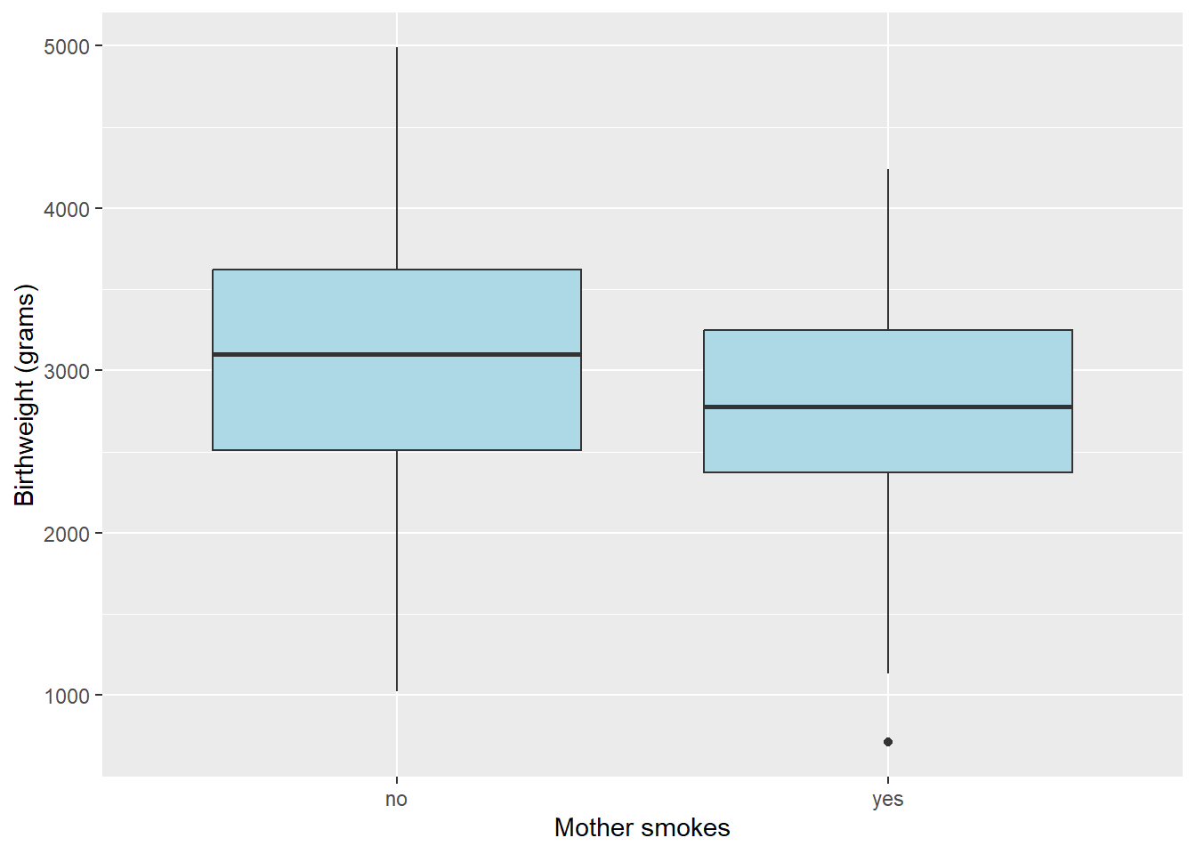
Compare birth-weight by smoking status, we can see that smoker babies are smaller, but there is overlap.
7.2.4 Differences in Birthweight by Smoking Status
How can we assess whether this difference is statistically significant?
Let’s compute a summary table
# Notice the consistent use of round() to ensure that our summaries
# do not have too many decimal values
birthwt %>%
  group_by(mother.smokes) %>%
  summarize(mean.birthwt = round(mean(birthwt.grams), 0),
            sd.birthwt = round(sd(birthwt.grams), 0))
## # A tibble: 2 × 3
## mother.smokes mean.birthwt sd.birthwt
## <fct> <dbl> <dbl>
## 1 no 3056 753
## 2 yes 2772 6607.2.5 Differences in Birthweight by Smoking Status
The standard deviation is good to have, but to assess statistical significance we really want to have the standard error.
Let’s compute a summary table
birthwt %>%
  group_by(mother.smokes) %>%
  summarize(num.obs = n(),
            mean.birthwt = round(mean(birthwt.grams), 0),
            sd.birthwt = round(sd(birthwt.grams), 0),
            se.birthwt = round(sd(birthwt.grams) / sqrt(num.obs), 0))
## # A tibble: 2 × 5
## mother.smokes num.obs mean.birthwt sd.birthwt se.birthwt
## <fct> <int> <dbl> <dbl> <dbl>
## 1 no 115 3056 753 70
## 2 yes 74 2772 660 77If we use a confidence interval around the sample means, there is less overlap between the two groups. \[\bar{x}\pm se*t_{\alpha /2} \]
7.2.6 T-test for Birthweight by Smoking Status
In this case study, we have been looking at a sample of mothers, some who smoke and some who do not. These are samples and not populations. Therefore, we need to use a two sample t-test.
This difference is looking quite significant. To run a two-sample t-test, we can simple use the t.test() function.
##
##  Welch Two Sample t-test
##
## data:  birthwt.grams by mother.smokes
## t = 2.7299, df = 170.1, p-value = 0.007003
## alternative hypothesis: true difference in means between group no and group yes is not equal to 0
## 95 percent confidence interval:
##   78.57486 488.97860
## sample estimates:
##  mean in group no mean in group yes
##          3055.696          2771.919
7.2.7 Interpreting Output
There are a few things from the output we can note.
First, is the p-value. The p-value tells us the likelihood that the null hypothesis (in this case no difference between groups) is true. For p-values less than 5 percent, we can reject the null hypothesis and state there is a statistically significant difference between the two groups.
The p-value in our t-test was 0.0070025, which is less than 1 percent so we can reject the null hypothesis.
Our study finds that birth weights are on average higher in the non-smoking group compared to the smoking group (t-statistic 2.73, p=0.007, 95 % CI [78.6, 489]g)
7.3 Standard Levels of significance
Levels of significance, \(\alpha\), are commonly - \(\alpha\) = 0.10 is marginally significant - \(\alpha\) = 0.05 is significant - \(\alpha\) = 0.01 is very significant
We reject the null hypothesis \(H_0\) if the p-value \(< \alpha\).
The significance level represents the probability of committing a Type I error that we are willing to accept. A Type I error is rejecting the null hypothesis when the null hypothesis is true.
7.4 Warning
7.4.1 Can We Accept the Null Hypothesis?
Some researchers say that a hypothesis test can have one of two outcomes: you accept the null hypothesis or you reject the null hypothesis. Many statisticians, however, take issue with the notion of “accepting the null hypothesis.” Instead, they say: you reject the null hypothesis or you fail to reject the null hypothesis.
Why the distinction between “acceptance” and “failure to reject?” Acceptance implies that the null hypothesis is true. Failure to reject implies that the data are not sufficiently persuasive for us to prefer the alternative hypothesis over the null hypothesis.
Think of it this way. In court, we say a person is either guilty or not guilty. We do not say the person is innocent. That is, we conclude that either there is enough evidence to say the person is guilty or there isn’t enough evidence (fail to reject).