Chapter 18 Count Models
In these notes, we will discuss several types of count models
- Ordered Probit/Logit
- Poisson Model
- Negative Binomial
- Hurdle Model
- Zero Inflated Poisson Model
18.1 Oridinal Categorical Variables
Suppose your dependent is categorical in nature and these categories show an ordinal proper (i.e. you can order them)
Examples: Surveys including Likert Scales (strongly agree, agree, neither, disagree, strongly disagree)
Medalling in the Olympics (Gold, Silver, Bronze)
Soda size preference (small, medium, large, extra large)
18.2 Ordered Probit/Logit
In these cases of ordinal categorical variables, we use an ordered probit/logit model.
Notice, these responses, while they can be ordered, the distance between levels is not constant.
That is, we do not know what increase is necessary to move someone from strongly disagree to just disagree.
18.2.1 Ordered Probit/Logit Math
The math of the ordered probit/logit is very similar to a simple binary model
There is just one difference, we need to estimate level parameters.
The math to the ordered probit/logit is very similar to a simple binary model
There is just one difference, we need to estimate level parameters.
Consider three observed outcomes: y = 0,1,2. Consider the latent variable model without a constant: \[y^{*} = \beta_1 x_1 +...+\beta_k x_k +\epsilon\] where \(\epsilon \rightarrow N(0,1)\). Define two cut-off points: \(\alpha_1 < \alpha_2\) We do not observe \(y^{*}\), but we do observe choices according to the following rule
- y = 0 if \(y^{*} < \alpha_1\);
- y = 1 if \(\alpha_1 < y^{*} < \alpha_2\);
- y = 2 if \(\alpha_2 < y^{*}\)
18.2.2 Analytical Example
y = 0 if inactive, y = 1 if part-time, and y = 2 if full-time
\(y* = \beta_e educ +\beta_k kids +\epsilon\), where \(\epsilon \rightarrow N (0,1)\)
Then y = 0 if \(\beta_e educ +\beta_k kids +\epsilon\) < \(\alpha_1\)
y = 1 if \(\alpha_1 < \beta_e educ +\beta_k kids +\epsilon\) < \(\alpha_2\)
y = 2 if \(\alpha_2 < \beta_e educ +\beta_k kids +\epsilon\)
We could alternatively introduce a constant \(\beta_0\) and assume that \(\alpha_1\) = 0.
18.2.3 Log Likelihood Function
\[Log \, L=\sum_{i=1}^{n} \sum_j Z_{ij}[F_{ij}-F_{ij-1}]\]
where \(F_{ij}=F(\alpha_j-\beta_e educ -\beta_k kids)\) and \(Z_{ij}\) is an indicator that equals 1 if person i select option j and zero otherwise.
We choose the values of \(\alpha\) and \(\beta\) that maximize the value of the log likelihood function.
However, in the case of models such as ordered probit and ordered logit failure to account for heteroskedasticity can lead to biased parameter estimates in addition to misspecified standard errors
18.2.4 Ordered Logit in R
A study looks at factors that influence the decision of whether to apply to graduate school.
College juniors are asked if they are unlikely, somewhat likely, or very likely to apply to graduate school.
Hence, our outcome variable has three categories.
Data on parental educational status, whether the undergraduate institution is public or private, and current GPA is also collected.
18.2.5 Example: Data
##             apply pared public  gpa
## 1     very likely     0      0 3.26
## 2 somewhat likely     1      0 3.21
## 3        unlikely     1      1 3.94
## 4 somewhat likely     0      0 2.81
## 5 somewhat likely     0      0 2.53
## 6        unlikely     0      1 2.59
## one at a time, table apply, pared, and public
lapply(dat[, c("apply", "pared", "public")], table)## $apply
##
## unlikely somewhat likely very likely
## 220 140 40
##
## $pared
##
## 0 1
## 337 63
##
## $public
##
## 0 1
## 343 57library(MASS)
m <- polr(apply ~ pared + public + gpa, data = dat, Hess=TRUE)
## view a summary of the model
summary(m)## Call:
## polr(formula = apply ~ pared + public + gpa, data = dat, Hess = TRUE)
##
## Coefficients:
## Value Std. Error t value
## pared 1.04769 0.2658 3.9418
## public -0.05879 0.2979 -0.1974
## gpa 0.61594 0.2606 2.3632
##
## Intercepts:
## Value Std. Error t value
## unlikely|somewhat likely 2.2039 0.7795 2.8272
## somewhat likely|very likely 4.2994 0.8043 5.3453
##
## Residual Deviance: 717.0249
## AIC: 727.024918.2.6 Predicting probabailities
Let’s say we want to know the probability that someone who’s parents are educated is likely very likely to go to graduate school.
We want to know \[Pr(y=2|pared=1, public=0)\]
18.2.7 Calculating probabilities
## First let's find the cumulative probability of being less than 2.
gpa<-as.vector(seq(0,4,.1))
pared.f<-rep(1,length(gpa))
public.f<-rep(0,length(gpa))
fakedata=as.matrix(rbind(pared.f,public.f,gpa))
p2=exp(m$zeta[2]-t(fakedata)%*%m$coefficients)/(1+exp(m$zeta[2]
                +t(fakedata)%*%m$coefficients))
## but we want to know Pr(y=2)=1-Pr(y<2)
p2=1-p2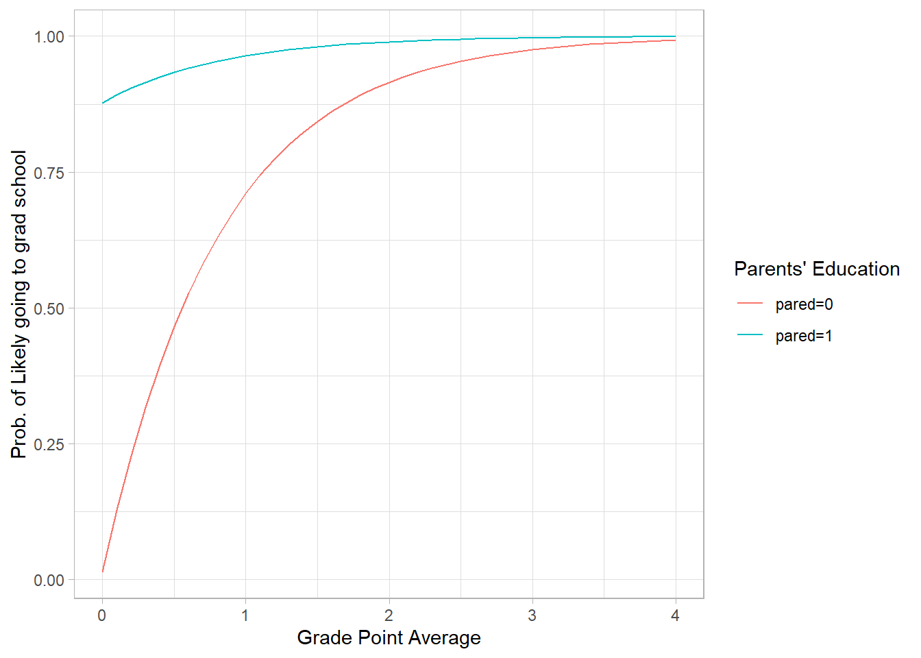
18.2.8 Marginal Effects
Re-run the example from the notes, but this time using the oglmx package
library(oglmx)
m_probit <- oprobit.reg(apply ~ pared + public + gpa, data = dat)
m_logit <- ologit.reg(apply ~ pared + public + gpa, data = dat)
m1_probit<-margins.oglmx(m_probit)
m1_logit<-margins.oglmx(m_logit)
## Marginal Effects on Pr(Outcome==unlikely)
## Marg. Eff Std. error t value Pr(>|t|)
## pared -0.234412 0.059115 -3.9654 7.328e-05 ***
## public -0.004024 0.068454 -0.0588 0.95312
## gpa -0.141735 0.062020 -2.2853 0.02229 *
## ------------------------------------
## Marginal Effects on Pr(Outcome==somewhat likely)
## Marg. Eff Std. error t value Pr(>|t|)
## pared 0.1076629 0.0229564 4.6899 2.734e-06 ***
## public 0.0023484 0.0398268 0.0590 0.95298
## gpa 0.0829761 0.0373413 2.2221 0.02628 *
## ------------------------------------
## Marginal Effects on Pr(Outcome==very likely)
## Marg. Eff Std. error t value Pr(>|t|)
## pared 0.1267493 0.0417507 3.0359 0.002398 **
## public 0.0016756 0.0286283 0.0585 0.953328
## gpa 0.0587591 0.0261803 2.2444 0.024807 *
## ---
## Signif. codes: 0 '***' 0.001 '**' 0.01 '*' 0.05 '.' 0.1 ' ' 1## Marginal Effects on Pr(Outcome==unlikely)
## Marg. Eff Std. error t value Pr(>|t|)
## pared -0.254585 0.060090 -4.2368 2.268e-05 ***
## public 0.014492 0.073372 0.1975 0.84343
## gpa -0.152406 0.064485 -2.3634 0.01811 *
## ------------------------------------
## Marginal Effects on Pr(Outcome==somewhat likely)
## Marg. Eff Std. error t value Pr(>|t|)
## pared 0.1374769 0.0285199 4.8204 1.433e-06 ***
## public -0.0096968 0.0494695 -0.1960 0.84460
## gpa 0.1012240 0.0439337 2.3040 0.02122 *
## ------------------------------------
## Marginal Effects on Pr(Outcome==very likely)
## Marg. Eff Std. error t value Pr(>|t|)
## pared 0.1171084 0.0387096 3.0253 0.002484 **
## public -0.0047951 0.0239160 -0.2005 0.841092
## gpa 0.0511818 0.0222472 2.3006 0.021414 *
## ---
## Signif. codes: 0 '***' 0.001 '**' 0.01 '*' 0.05 '.' 0.1 ' ' 118.3 Poisson and Negative Binomial Model
Count data are integer counts of the outcome variable that can include the number zero.
These data present problems for typical linear regression methods because the outcome variable is non-negative, but the regression error is bounded by \(-\infty\) and \(\infty\).
We cannot simply take a the natural log of the outcome variable because zero’s are present.
Also, the integer values are more discrete in nature.
18.3.1 Examples of count data
Count data capture the number of occurrences over a fixed time intervals such as:
- Number of Suicides in a state over a year
- Number of cars served through a fast food drive thru in a day
- Number of children in a family
- Number of doctors visits
- Number of website visitors
18.3.2 Poisson Distribution
The Poisson density function is \[Pr(Y=y)=\frac{e^{-\lambda}\lambda^y}{y!}\]
where the \(E[y|X]=Var[y|X]=\lambda\)
For our purposes, we assume \(\lambda=exp(X\beta)\)
Interpretation of \(\beta\) is the percentage change in \(\lambda\) for a one unit increase in \(X\).
18.3.3 Properties of the Poisson Distribution
The equidispersion property of the Poisson distribution: Implies \(E[y|X]=Var[y|X]=\lambda\), which is very often violated.
When this property fails to hold, we state that there is overdispersion in the data. In this case, the negative binomial can be used.
Overdispersion causes the standard errors estimated using the Poisson distribution to be too small. An alternative approach is to estimate heterosckedastic (robust) standard errors.
Woolridge (1999) had demonstrated that using robust standard errors compensates for the overdispersion problem and often performs better than the negative binomial distribution.
18.3.4 Negative Binomial Distribution
The Negative Binomial distribution has a less restrictive relationship between the mean and variance of y. \[Var(y)=\lambda+\alpha \lambda^2\]
We can think of \(\alpha\) as the overdispersion parameter.
18.3.5 Testing for Overdispersion
Step 1. Estimate the count model using the negative binomial distribution.
Step 2. Test \(H_o:\alpha=0\) vs \(H_a:\alpha\neq0\)
Step 3. Determine which case you are in
- If \(\alpha=0\), then the Poisson model holds
- If \(\alpha>0\), then we have overdispersion (very common)
- If \(\alpha<0\), then we have underdispersion (rare)
18.3.6 Poisson and Negative Binomial in R
library(MASS); library(AER) #MASS contains the negative binomial model
data("NMES1988")
plot(table(NMES1988$visits),xlab="Physician Office Visits", ylab="Counts")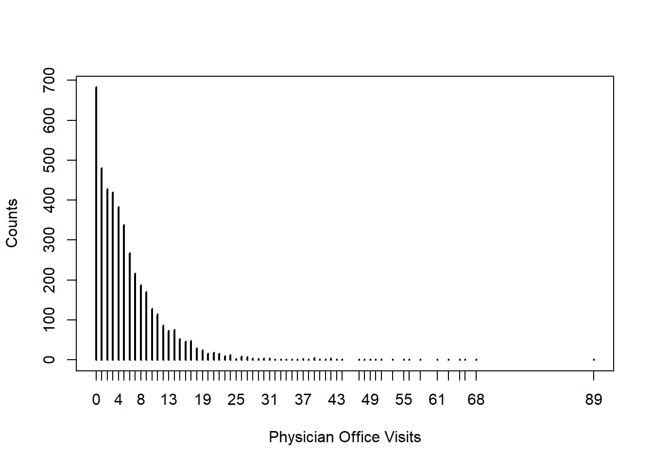
18.3.7 Issues with the data
First, notice the shape of Physician office visits. Does this look normally distributed to you?
Should we be concerned with the mass of zero’s?
How about those outliers?
18.3.8 Standard Poisson and Negative Binomial Model
pformu<-visits~hospital+chronic+insurance+gender+school
fm_pois <- glm(pformu, data = NMES1988, family = poisson)
cov.m1 <- vcovHC(fm_pois, type="HC0")
std.err <- sqrt(diag(cov.m1))
fm_qpois <- glm(pformu, data = NMES1988, family = quasipoisson)
fm_nbin <- glm.nb(pformu, data = NMES1988)
texreg::htmlreg(list(fm_pois,fm_pois,fm_qpois,fm_nbin),custom.model.names = c("Poisson","Poisson Robust","Quasi Poisson","Neg. Bin"), override.se = list(NULL,std.err,NULL,NULL), single.row = TRUE, custom.coef.names = c("Intercept","Hospital","Chronic","Insurance Eyes","School","Male","Theta"))| Poisson | Poisson Robust | Quasi Poisson | Neg. Bin | |
|---|---|---|---|---|
| Intercept | 1.05 (0.02)*** | 1.05 (0.06)*** | 1.05 (0.06)*** | 0.99 (0.05)*** |
| Hospital | 0.18 (0.01)*** | 0.18 (0.02)*** | 0.18 (0.02)*** | 0.24 (0.02)*** |
| Chronic | 0.17 (0.00)*** | 0.17 (0.01)*** | 0.17 (0.01)*** | 0.20 (0.01)*** |
| Insurance Eyes | 0.18 (0.02)*** | 0.18 (0.04)*** | 0.18 (0.04)*** | 0.19 (0.04)*** |
| School | -0.12 (0.01)*** | -0.12 (0.04)*** | -0.12 (0.03)*** | -0.14 (0.03)*** |
| Male | 0.02 (0.00)*** | 0.02 (0.00)*** | 0.02 (0.00)*** | 0.02 (0.00)*** |
| AIC | 36314.70 | 36314.70 | 24430.49 | |
| BIC | 36353.05 | 36353.05 | 24475.22 | |
| Log Likelihood | -18151.35 | -18151.35 | -12208.24 | |
| Deviance | 23527.28 | 23527.28 | 23527.28 | 5046.63 |
| Num. obs. | 4406 | 4406 | 4406 | 4406 |
| ***p < 0.001; **p < 0.01; *p < 0.05 | ||||
18.3.9 Fixed Effects Poisson
library(pglm)
library(readstata13)
library(lmtest)
library(MASS)
ships<-readstata13::read.dta13("http://www.stata-press.com/data/r13/ships.dta")
ships$lnservice=log(ships$service)
res <- glm(accident ~ op_75_79+co_65_69+co_70_74+co_75_79+lnservice,family = poisson, data = ships)
res1 <- pglm(accident ~ op_75_79+co_65_69+co_70_74+co_75_79+lnservice,family = poisson, data = ships, effect = "individual", model="within", index = "ship")
##
## z test of coefficients:
##
## Estimate Std. Error z value Pr(>|z|)
## (Intercept) -5.22294 0.48261 -10.8224 < 2.2e-16 ***
## op_75_79 0.35465 0.11685 3.0351 0.002404 **
## co_65_69 0.67352 0.15029 4.4814 7.417e-06 ***
## co_70_74 0.79669 0.17019 4.6811 2.853e-06 ***
## co_75_79 0.39785 0.23375 1.7020 0.088746 .
## lnservice 0.83107 0.04602 18.0591 < 2.2e-16 ***
## ---
## Signif. codes: 0 '***' 0.001 '**' 0.01 '*' 0.05 '.' 0.1 ' ' 1##
## z test of coefficients:
##
## Estimate Std. Error z value Pr(>|z|)
## op_75_79 0.37026 0.11815 3.1339 0.001725 **
## co_65_69 0.66254 0.15364 4.3124 1.615e-05 ***
## co_70_74 0.75974 0.17766 4.2763 1.900e-05 ***
## co_75_79 0.36974 0.24584 1.5040 0.132589
## lnservice 0.90271 0.10180 8.8672 < 2.2e-16 ***
## ---
## Signif. codes: 0 '***' 0.001 '**' 0.01 '*' 0.05 '.' 0.1 ' ' 118.4 Excessive Zeros
A problem that plagues both the Poisson and Negative Binomial Models is when there are excessive zeros in the data.
There a two approaches to address these zeros
Hurdle Model (aka Two Part Model)
Zero Inflated Model
18.4.1 Hurdle Model

The Hurdle Model treats the distribution of zeros separately from the distribution of positive values.
For example, your choice to start exercising may be different than your choice about how often to exercise.
The first part of the model is typical captured by a probit or logit model.
The second part of the model is captured by a poisson or negative binomial model that is truncated at 1.
Let the process generating the zeros be \(f_1(0)\) and the process generating the positive responses be \(f_2(0)\), then the two part density distribution is \[g(y)=\left\{\begin{matrix} f_1(0) & y=0 \\ \frac{1-f_1(0)}{1-f_2(0)}f_2(y) & y>0 \end{matrix}\right.\]
If \(f_1(0)=f_2(0)\), then the hurdle model reduces to the standard count model.
18.4.2 Zero Inflated Model
The zero inflated model treats zeros differently than the hurdle model.
Zeros are produce for two reasons.
There is an exogenous mass of zeros that are independent of the count process.
There are a set of zeros that are caused by the count process.
Example: You may drink alcohol or you may not. Even if you do drink alcohol you may not drink alcohol everyday. On the days you do drink, you may have 1, 2, 3 or more drinks.
Let the process generating the structural zeros be \(f_1(.)\) and the process generating the random counts including zero be \(f_2(.)\), then the two part density distribution is
\[g(y)=\left\{\begin{matrix} f_1(0)+(1-f_1(0))f_2(0) & y=0 \\ (1-f_1(0))f_2(y) & y>0 \end{matrix}\right.\]
Think of this model as a finite mixture of a zero mass and the count model.
Next, we will use R to estimate these models.
The package you will need is pscl: zero-inflation and hurdle models via zeroinfl() and hurdle()
18.4.3 Hurdle Model and Zero Inflated Model in R
library(pscl)
dt_hurdle <- hurdle(visits ~ hospital + chronic + insurance + school + gender |
 hospital + chronic + insurance + school + gender,
 data = NMES1988, dist = "negbin")
dt_zinb <- zeroinfl(visits ~ hospital + chronic + insurance + school + gender |
+ hospital + chronic + insurance + school + gender,
 data = NMES1988, dist = "negbin")
texreg::htmlreg(list(dt_hurdle,dt_zinb), single.row = TRUE, omit.coef = "Zero", custom.coef.names = c("Intercept","Hospital","Chronic","Insurance Eyes","School","Male","Theta"))| Model 1 | Model 2 | |
|---|---|---|
| Intercept | 1.26 (0.06)*** | 1.25 (0.06)*** |
| Hospital | 0.24 (0.02)*** | 0.22 (0.02)*** |
| Chronic | 0.15 (0.01)*** | 0.16 (0.01)*** |
| Insurance Eyes | 0.06 (0.04) | 0.10 (0.04)* |
| School | 0.01 (0.00)** | 0.02 (0.00)*** |
| Male | -0.08 (0.03)* | -0.09 (0.03)** |
| Theta | 0.30 (0.04)*** | 0.37 (0.03)*** |
| AIC | 24277.81 | 24278.15 |
| Log Likelihood | -12125.90 | -12126.07 |
| Num. obs. | 4406 | 4406 |
| ***p < 0.001; **p < 0.01; *p < 0.05 | ||