Chapter 19 Censored and Truncated Data
19.1 Censored Data
In the world of data science sometimes data do not appear the way we would like.
One such case is when data are either top coded or bottom coded.
For example, you may be interested in household income. You run to the American Community Survey only to find the following.
- Household earning less than $10,000 are given a lumped into one income category (i.e. bottom coded).
- Household earning more than $1,000,000 are given a lumped into the top income category (i.e. top coded).
These variables are missing due to exogenous reasons.
A second type of censored data is when the data are missing for endogenous reasons.
For example, a person’s wage information is missing because they are not in the labor force. However, this does not mean that if we could magically put them in the labor force that their wage would be zero.
Simply, the person’s reservation wage is higher than the wage offers they are receiving.
A different example, consider you want to know the effect of High School GPA on College GPA. You will only observe a college GPA for people who get into college. Likewise, if you sample college students, then you will observe college GPA, but you will only observe the high school GPA of individuals who entered college.
Truncated Data
A third problem that can exist is that not only can you not observe the dependent variable, but you also cannot observed the explanatory variables.
In this case, if both the dependent and independent variables are censored due to a cutoff value, then we say the data are truncated.
Therefore, we need three different types of models to deal with exogenous missing data and endogenous missing data.
Tobit - exogenously censored dependent variable.
Truncated Regression - exogenous censoring of both dependent and independent variables.
Sample Selection Model (Heckman Model) - endogenously censored dependent variable
19.2 Tobit
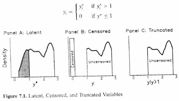
Suppose Y (wages) are subject to “top coding” (as is often observed in government data): \[Y=\left\{\begin{matrix} y^* & y^*<c \\ c & y^*>c \end{matrix}\right.\]
We are interested in estimating the equation \[Y=X\beta+u\]
If we are willing to assume \(u \rightarrow N(0,\sigma^2)\), then we can use the Tobit Model
19.2.1 Tobit Density and Likelihood Function
The probability density of Y will resemble that of a normal distribution. \[f(y)=\left\{\begin{matrix} \frac{1}{\sigma}\phi(\frac{y_i-X_i'beta}{\sigma}) & y^*<c \\ 1-\Phi(\frac{c-X_i'beta}{\sigma}) & y^*>c \end{matrix}\right.\]
Log Likelihood Function \[LL(\beta,\sigma)=\sum_{c>y} \frac{1}{\sigma}\phi(\frac{y_i-X_i'beta}{\sigma})+\sum_{c<y} 1-\Phi(\frac{c-X_i'beta}{\sigma})\]
19.2.2 Bottom Coding
The equation is very similar for the bottom coding situation. Bottom coding means we are censored from below. \[Y=\left\{\begin{matrix} y^* & y^*>c \\ c & y^*<c \end{matrix}\right.\] The likelihood function changes to capture this difference in bottom coding Log Likelihood Function \[LL(\beta,\sigma)=\sum_{c<y} \frac{1}{\sigma}\phi(\frac{y_i-X_i'beta}{\sigma})+\sum_{c>y} \Phi(\frac{c-X_i'beta}{\sigma})\]
19.2.3 The Expected Value of the Tobit model
Let’s assume your y variable is bottom coded at zero. This means we only observe Y if Y>0.
The unconditional expected value is of Y is \[E[Y_i]=\Phi(\frac{x_i \beta}{\sigma})(x_i \beta+\sigma *\lambda) \\ \lambda = \frac{\phi(x_i \beta)/\sigma}{\Phi(x_i \beta/\sigma)}\] If we condition on Y>0, then the expected value simplifies to
\[E[Y_i|Y_i>0,x]=x_i \beta+\sigma *\lambda \\ \lambda = \frac{\phi(x_i \beta)/\sigma}{\Phi(x_i \beta/\sigma)}\] The \(\lambda\) term is the Inverse Mills Ratio.
19.2.4 Marginal Effects of Tobit Model
We can calculate the probability of Y>0 \[Pr(Y>0)=\Phi(x_i \beta/\sigma) \\ \frac{d Pr(Y>0)}{dx} = \frac{\beta}{\sigma}*\phi(x_i \beta/\sigma)\] Similarly, we can calculate the marginal effect of x on Y. \[\frac{d E[Y]}{dx} = \beta*\Phi(x_i \beta/\sigma)\]
19.2.5 Tobit Model in R
library(AER)
library(stargazer)
data("Affairs")
fm.ols <- lm(affairs ~ age + yearsmarried + religiousness + occupation
             + rating,  data = Affairs)
fm.tobit <- tobit(affairs ~ age + yearsmarried + religiousness + occupation
                  + rating,  data = Affairs)
fm.tobit2 <- tobit(affairs ~ age + yearsmarried + religiousness + occupation
                   + rating,  right = 4, data = Affairs)
stargazer(fm.ols,fm.tobit,fm.tobit2,type="html")| affairs | |||
| OLS | Tobit | ||
| age | -0.050b (0.022) | -0.179b (0.079) | -0.178b (0.080) |
| yearsmarried | 0.162a (0.037) | 0.554a (0.135) | 0.532a (0.141) |
| religiousness | -0.476a (0.111) | -1.686a (0.404) | -1.616a (0.424) |
| occupation | 0.106 (0.071) | 0.326 (0.254) | 0.324 (0.254) |
| rating | -0.712a (0.118) | -2.285a (0.408) | -2.207a (0.450) |
| Constant | 5.608a (0.797) | 8.174a (2.741) | 7.901a (2.804) |
19.2.6 Marginal effects with Tobit
Let’s use the censReg package to estimate the tobit model and get marginal effects.
library(censReg)
estResult <- censReg( affairs ~ age + yearsmarried + religiousness + occupation + rating, data = Affairs )
margEff(estResult) %>% kable()| x | |
|---|---|
| age | -0.04192089 |
| yearsmarried | 0.12953651 |
| religiousness | -0.39417189 |
| occupation | 0.07621840 |
| rating | -0.53413656 |
19.3 Truncated Regression
Truncated data differ from censored data in that we only observe y and x if y is above (below) a certain cutoff. In censored data, we always observed x.
Example: Hausman and Wise’s analysis of the New Jersey negative income tax experiment (Truncated Regression)
Goal: Estimate earnings function for low income individuals
Truncation: Individuals with earnings greater than 1.5 poverty level were excluded from the sample.
Two types of inference:
- Inference about entire population in presence of truncation
- Inference about sub-population observed
\[y_i=x_i'\beta+e_i, i=1, ..., n\] where the error term \(e_i \rightarrow N(0,\sigma^2)\)
Truncation from below: observe \(y_i\) and \(x_i\) if \(y_i>c\)
Truncation from above: observe \(y_i\) and \(x_i\) if \(y_i<c\)
19.3.1 Truncated Normal Distribution
Let X be a normally distributed random variable with mean \(\mu\) and variance \(\sigma^2\). Also, let there be a cutoff constant \(c\).
Then we can write the probability density function of X to be \[\begin{align*}f(X|X>c) &= \frac{f(x)}{Pr(X>c)}=\frac{f(x)}{1-F(c)} \\ \\&= \frac{\frac{1}{\sigma}\phi\frac{x-\mu}{\sigma}}{1-\Phi(\frac{c-\mu}{\sigma})}\end{align*}\]
19.3.2 Truncated Normal Distribution
The mean and variance are given by \[\begin{align*}E[X|X>c] &= \mu+\sigma \lambda(\frac{c-\mu}{\sigma}) \\ var(X|X>c) &= \sigma^2(1-\delta(\frac{c-\mu}{\sigma})) \end{align*}\]
where \(\lambda(x)=\frac{phi(x)}{1-Phi(x)}\) = Inverse Mills Ratio and \(\delta(x)=\lambda(x)(\lambda(x)-x),\,0<\delta(x)<1\)
19.3.3 Truncated Normal Distribution
Consequences of not accounting for the truncation is that you will overstate the mean and understate the variance. WHY?
We are throwing out lower values pushing the mean up.
We are throwing out values from the extreme part of the distribution, which means we have less variation in the remaining data.

Simply using Ordinary Least Squares will result in a bias.
Instead, we use maximum likelihood. We can correct for the missing data by dividing the probability density function by the Pr(y>c).
\[f(y|y>c) =\frac{\frac{1}{\sigma}\phi\frac{y-x'\beta}{\sigma}}{1-\Phi(\frac{c-x'\beta}{\sigma})}\] Notice that \(\int_c^\infty f(y|y>c) dy=1\)
Likelihood function \[L(\beta,\sigma^2|x,y)=\prod_i^n \frac{\frac{1}{\sigma}\phi\frac{y-x'\beta}{\sigma}}{1-\Phi(\frac{c-x'\beta}{\sigma})}\]
19.3.4 Truncated Regression in R
########################
## Artificial example ##
########################
## simulate a data.frame
set.seed(1071)
n <- 10000
sigma <- 4
alpha <- 2
beta <- 1
x <- rnorm(n, mean = 0, sd = 2)
eps <- rnorm(n, sd = sigma)
y <- alpha + beta * x + eps
d <- data.frame(y = y, x = x)
We simulated data for this example. The above code created the data for us. This means we know what the actual values of the parameters should be. The constant is equal to 2 and the slope is equal to 1. Let’s see how OLS fairs.
library(truncreg) # Truncated Regression package
## truncated response
d$yt <- ifelse(d$y > 1, d$y, NA)
## compare estimates for full/truncated/censored/threshold response
fm_full <- lm(y ~ x, data = d)
fm_ols <- lm(yt ~ x, data = d)
fm_trunc <- truncreg(yt ~ x, data = d, point = 1, direction = "left")
OLS vs Truncreg
| Dependent variable: | |||
| Full Data | Truncated | ||
| OLS | OLS | Trunc. Reg. | |
| x | 0.983a (0.020) | 0.462a (0.019) | 0.982a (0.046) |
| Constant | 2.022a (0.040) | 4.645a (0.037) | 1.964a (0.177) |
Notice, OLS does get the correct estimate when we can see the whole dataset. When we truncate the dataset, OLS is off by a lot! The Truncated Regression model is much closer to the true parameter values when using the truncated dataset.
group1<-rep("Normal",length(d$y))
group2<-rep("Truncated",length(d$yt))
data_1<-data.frame(c(d$y,d$yt),c(group1,group2))
names(data_1)<-c("Y","groups")
library(ggplot2)
ggplot(data_1, aes(x=Y, fill=groups)) +
     geom_density(alpha=.3)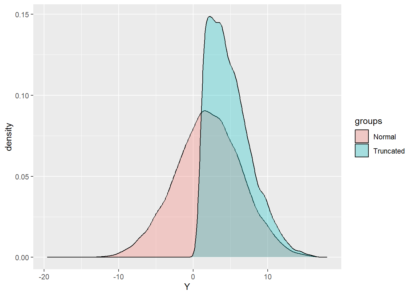
19.4 Endogenous Censoring
19.4.1 Examples of Endogenous Censoring
- Non-response Bias

Non-response bias is a type of bias that occurs in research studies, surveys, or polls when the responses of participants who choose not to respond differ from those who do respond. It is a form of selection bias that can lead to inaccurate or skewed results, as the non-respondents’ views or characteristics are not represented adequately in the data.
Non-response bias can arise in various situations, such as:
Surveys and Questionnaires: When a portion of the surveyed population chooses not to respond to a survey, the results may not accurately represent the entire population’s views or opinions.
Research Studies: In research studies that involve data collection from participants, if a significant number of participants refuse to participate or drop out during the study, the sample might not be representative of the target population, leading to biased findings.
Online Polls and Feedback: Non-response bias can also occur in online polls or feedback forms, where only a certain subset of individuals responds, potentially skewing the results.
Census and Demographic Data: In census data collection, if certain groups or individuals are more likely to avoid participating, the census results might not accurately reflect the true demographic makeup of the population.
The presence of non-response bias can undermine the validity and reliability of the findings, making it challenging to generalize the results to the entire population. Researchers and survey designers need to be aware of this bias and implement strategies to minimize its impact. Some common methods to address non-response bias include:
Incentives: Offering incentives to encourage participation can help increase response rates and reduce non-response bias.
Follow-up: Sending reminders and follow-up communications to non-respondents can sometimes improve response rates.
Weighting: Analyzing the characteristics of respondents and non-respondents and adjusting the data through weighting can help account for potential biases.
Sensitivity Analysis: Researchers can conduct sensitivity analyses to assess the impact of non-response on the study’s results and conclusions.
Overall, minimizing non-response bias is essential to ensure the accuracy and representativeness of research findings and survey results.
- Survivorship/Attrition Bias

Survivorship bias is a cognitive bias that occurs when we focus on the individuals or things that “survived” a particular process or event while overlooking those that did not. It often leads to a skewed or incomplete analysis because the data only includes the successful outcomes, leaving out the failures or less successful instances.
The concept of survivorship bias is well illustrated by the example of WWII planes. During World War II, the military analyzed the damage patterns on planes that returned from missions and used this information to reinforce and strengthen those areas. The reasoning was that if the planes survived and returned, those were the areas that needed improvement.
However, Abraham Wald, a mathematician, realized that survivorship bias was at work here. The military only considered the planes that made it back safely, ignoring the ones that were shot down or crashed. As a result, they were overlooking critical information from the failed planes, which might have revealed vulnerabilities or areas needing reinforcement. By focusing only on the surviving planes, they were not accounting for the full picture of what made an aircraft more likely to survive a mission.
Realizing this mistake, Wald suggested to place additional armor where there wasn’t any bullet holes. Wald induced that the other areas must have caused the planes not to return.
Survivorship bias is not limited to military contexts. It can be found in various fields, including finance, investing, business, and self-help. For instance, when studying successful entrepreneurs, only looking at the traits of successful individuals and ignoring those who failed can lead to oversimplified and misleading conclusions about the factors contributing to success.
Or considering only famous people who did not complete college like Mark Zuckerberg, Steve Jobs, and Bill Gates. We ignore the many, many, more people who dropped out of college and did not become famous.
To avoid survivorship bias, it is crucial to consider both the successes and the failures in any analysis or study to gain a more balanced and accurate understanding of the underlying factors and make well-informed decisions.

Here are some other examples of sample selection bias:
Volunteer Bias: In research studies or surveys where participation is voluntary, individuals who choose to participate may have different characteristics or opinions from those who do not volunteer. This can lead to an unrepresentative sample, as the characteristics of the participants may not reflect the broader population.
Convenience Sampling: Convenience sampling involves selecting individuals who are easy to reach or readily available, rather than using a random or systematic sampling method. This can lead to an unrepresentative sample, as those who are conveniently accessible may not represent the broader population accurately.
Attrition bias, also known as dropout bias, occurs in research studies when there is a systematic difference between participants who remain in the study until its completion and those who drop out or are lost to follow-up before the study concludes. It is a type of selection bias that can affect the internal validity of a study, as it may lead to biased and misleading results.
Attrition bias can arise in longitudinal studies, clinical trials, or any research where data is collected over an extended period.
Hawthorne Effect: The Hawthorne Effect refers to the alteration of behavior by study participants due to the awareness of being observed or studied. This can lead to biased results if the behavior observed during the study does not reflect the participants’ usual behavior.
Health Selection Bias: Health selection bias occurs when individuals’ health status influences their likelihood of being included in a study or survey. For example, in a health-related survey conducted via phone calls, healthier individuals may be more likely to answer the phone and participate, leading to biased results.
Pre-screening Bias: When researchers pre-screen potential participants based on certain criteria before selecting the final sample, it can lead to a biased sample. For instance, if only individuals above a certain income level are included, the sample may not represent the entire population accurately.
For example, let’s say that you want to know if High School GPA affects College GPA. You get the universe of College Students. You obtain both their high school GPA and their college GPA. Why is focusing on just this group a problem?
Colleges do not accept people randomly. Student applicants go through a screening process. Additionally, not all high school students go to college either by choice or because their aptitude scores are not high enough. Both of these restrictions create a bias.
To minimize sample selection bias, researchers should use random sampling techniques whenever possible and be cautious about potential sources of bias in their sampling methods. Ensuring a representative sample is essential to draw accurate and generalizable conclusions from research studies and surveys.
19.4.2 Heckman Model
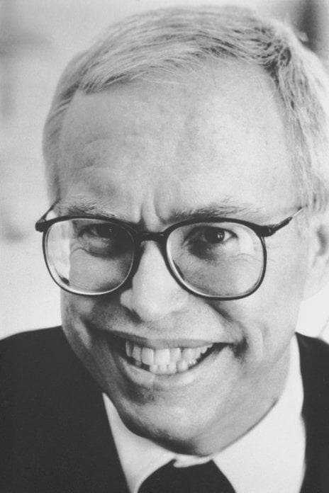
James Heckman developed a simple method to deal with sample selection problems. For his efforts, he was recognized with The Sveriges Riksbank Prize in Economic Sciences in Memory of Alfred Nobel in 2000.
The Heckman model, also known as the Heckit model or selection model, is an econometric technique used to address sample selection bias in statistical analysis. It was developed by economist James J. Heckman in the late 1970s and has since become widely used in various fields, especially in economics and social sciences.
The Heckman model aims to correct this bias by explicitly modeling the selection process and jointly estimating the selection equation and the outcome equation. The model is typically used when the sample can be divided into two groups: those selected (participating) and those not selected (non-participating).
The Heckman model consists of two main equations:
Selection Equation: This equation models the probability of selection into the sample. It is typically estimated using a probit or logit model and includes variables that influence the selection process. The dependent variable in this equation is a binary indicator variable, indicating whether an observation is selected (1) or not selected (0).
Outcome Equation: This equation models the outcome of interest, such as wages, employment status, or any other dependent variable. It includes the selection variable from the selection equation as an additional explanatory variable to account for the selection bias. The outcome equation is estimated using ordinary least squares (OLS) or other relevant regression techniques.
The key assumption in the Heckman model is the presence of an exclusion restriction. This means that there must be at least one variable that affects the selection process but does not directly influence the outcome variable. This variable is typically included in the selection equation but not in the outcome equation.
By jointly estimating the selection equation and the outcome equation, the Heckman model allows researchers to obtain consistent estimates for the coefficients in the outcome equation, accounting for the selection bias. The model also provides the Heckman correction term, which quantifies the extent of the selection bias and can be used to adjust the estimates for unbiased results.
The Heckman model is particularly useful when dealing with non-random samples and can help improve the accuracy of estimations in situations where sample selection bias might be a concern. However, it is essential to meet the model’s assumptions, including the exclusion restriction, for valid and reliable results.
19.5 The Two-Step Method
The Heckman Model can be thought of as a two part model (but it can be done in one step)
Step 1. You estimate a probit/logit model that determines if the dependent variable is censored.
Step 2. Construct the Inverse Mills Ratio (corrects for sample selection)
Step 3. Run the regression including the Inverse Mills Ratio as an explanatory variable.
Heckman Model: Math
Consider the model \[\begin{align*}Y &= X\beta +\sigma u \\ d &=1(z'\gamma+v>0) \end{align*}\]
where z contains an instrumental variable not contained in X. The error terms \(v\) and \(u\) are assumed to be jointly distributed standard normal. \[\binom{u}{v}\to N\left ( 0,\begin{bmatrix} 1 & \rho \\ \rho & 1 \end{bmatrix} \right )\]
We want to estimate the
\[\begin{align*}E[Y|X,d=1] &= X\beta+\sigma E[u|d=1] \\ &= X\beta+\sigma E[u|z'\gamma+v>0] \\ &= X\beta+\sigma \rho \lambda(z'\gamma) \end{align*}\]
where \(\lambda(z\gamma)\) is called the Inverse Mills Ratio \[\lambda(z\gamma)=\frac{\phi(z'\gamma)}{\Phi(z'\gamma)}\] Notice, this is the ratio between the normal pdf and the normal cdf of our probit coefficients with the person’s X’s.
19.5.1 Heckman Two Step
First, we estimate the decision equation to get our estimates of \(\gamma\).
We use those estimates to construct \(\lambda(z'\widehat{\gamma})\).
Then we estimate the level equation as \[Y=X\beta+\alpha\lambda(z'\widehat{\gamma})+u\]
If \(\alpha=0\), then there is no sample selection problem.
OLS versus Heckman
Now is a good time to think about how Heckman corrects OLS.
Let’s restate the omitted variable bias (OVB) table, but using the correction factor as the OV. If x affects both the participation equation and the level equation, then we will have some sort of OVB.
| Signs | \(Corr(x,\text{Mills Ratio})>0\) | \(Corr(x,\text{Mills Ratio})<0\) |
|---|---|---|
| \(\alpha>0\) | Positive Bias | Negative Bias |
| \(\alpha<0\) | Negative Bias | Positive Bias |
19.5.2 Simulation Example
library(tidyverse)
library(sampleSelection)
set.seed(123456)
N = 10000
educ = sample(1:16, N, replace = TRUE)
age  = sample(18:64, N, replace = TRUE)
covmat = matrix(c(.46^2, .25*.46, .25*.46, 1), ncol = 2)
errors = mvtnorm::rmvnorm(N, sigma = covmat)
z = rnorm(N)
e = errors[, 1]
v = errors[, 2]
wearnl = 4.49 + .08 * educ + .012 * age + e
d_star = -1.5 + 0.15 * educ + 0.01 * age + 0.15 * z + v

observed_index  = d_star > 0
d = data.frame(wearnl, educ, age, z, observed_index)
# lm based on full data
lm_all = lm(wearnl ~ educ + age, data=d)

# lm based on observed data
lm_obs = lm(wearnl ~ educ + age, data=d[observed_index,])
# Sample Selection model
selection_2step = selection(observed_index ~ educ + age + z, wearnl ~ educ + age, method = '2step')
Again, we will use simulation methods to demonstrate the power of these models when done correctly.
The actual wage equation is given by the following equation. \[wearnl = 4.49 + .08 * educ + .012 * age + e\]
However, we only observe your wage if you decide to work. Your choice to work is dependent not only on the characteristics about the job, but also some non-work related characteristics.
\[d^* = -1.5 + 0.15 * educ + 0.01 * age + 0.15 * z + v\]
The decision equation is given above. When \(d^*>0\) you will work, otherwise you will stay unemployed.
In economics, the idea of people receiving the same job offer, but making different decisions on whether or not to work is based on the idea of a reservation wage.
The reservation wage is a concept used in labor economics to describe the minimum wage level at which an individual is willing to accept a job offer and enter the workforce. It represents the point at which the individual is indifferent between accepting employment and remaining unemployed.
When a person is unemployed and seeking a job, they will typically have a certain level of minimum wage in mind that they would be willing to accept for a particular job. This minimum wage is their reservation wage. If a job offer meets or exceeds their reservation wage, they are likely to accept the offer and start working. If the offer falls below their reservation wage, they may choose to continue searching for a better opportunity or remain unemployed.
Several factors influence an individual’s reservation wage, including:
Personal Financial Needs: The individual’s financial obligations, living expenses, and desired standard of living play a significant role in determining their reservation wage. Higher financial needs may lead to a higher reservation wage.
Skills and Education: A person’s level of education, work experience, and skills impact their perceived value in the job market. Individuals with more valuable and in-demand skills may have a higher reservation wage.
Job Market Conditions: The state of the job market, including the availability of job opportunities and the prevailing wages, can influence an individual’s reservation wage. In a tight job market with more demand for workers, individuals may be more inclined to set a higher reservation wage.
Unemployment Benefits: The availability and generosity of unemployment benefits can influence an individual’s reservation wage. Higher unemployment benefits may lead to a higher reservation wage, as individuals may be less willing to accept a low-paying job if they are receiving sufficient financial support through unemployment benefits.
The concept of the reservation wage is essential for understanding labor market dynamics, unemployment rates, and wage negotiations. It also helps economists and policymakers analyze the effects of changes in labor market conditions and government policies on the labor force participation and unemployment rates.
| wearnl | |||
| OLS | selection | ||
| educ | 0.080a (0.001) | 0.071a (0.001) | 0.078a (0.005) |
| age | 0.012a (0.0003) | 0.011a (0.0004) | 0.012a (0.001) |
| Constant | 4.469a (0.017) | 4.671a (0.026) | 4.516a (0.107) |
| N | 10,000 | 5,520 | 10,000 |
| rho | 0.210 | ||
| Inverse Mills Ratio | 0.096 (0.064) | ||
| Notes: | ***Significant at the 1 percent level. | ||
| **Significant at the 5 percent level. | |||
| *Significant at the 10 percent level. | |||
We can see that the Heckman model was able to recover both the wage equation parameters (or at least pretty close) and even the selection equation parameters.
Now, let’s apply the model to a real example. We use data from Mroz (1987), who studied the decision of married women to work.
Mroz, T. (1987) “The sensitivity of an empirical model of married women’s hours of work to economic and statistical assumptions”, Econometrica, 55, 765-799.
library(sampleSelection)
data( Mroz87 )
Mroz87$kids  <- ( Mroz87$kids5 + Mroz87$kids618 > 0 )
# Two-step estimation
# heckit(first stage equation, second stage equation, data, method c("2step","ml"))
heck.m1 <- heckit( lfp ~ age + I( age^2 ) + faminc + kids + educ,
   wage ~ exper + I( exper^2 ) + educ + city, Mroz87, method = "2step" )
# MLE Estimator
heck.m2 <- heckit( lfp ~ age + I( age^2 ) + faminc + kids + educ,
   wage ~ exper + I( exper^2 ) + educ + city, Mroz87, method = "ml" )
# OLS Estimator
ols.m1 <- lm(wage ~ exper + I( exper^2 ) + educ + city, Mroz87)
stargazer::stargazer(ols.m1,heck.m1,heck.m2,type="html", model.numbers = FALSE, font.size = "small", single.row = TRUE, star.char = c("c","b","a"), omit.table.layout = "sn")
Although not statistically significant, we can see there is a negative coefficient with respect to the mills ratio in the wage equation. Women who were more likely to accept the job had a lower reservation wage.
| wage | |||
| OLS | Heckman | ||
| selection | |||
| exper | 0.032 (0.062) | 0.021 (0.062) | 0.028 (0.062) |
| I(exper2) | -0.0003 (0.002) | 0.0001 (0.002) | -0.0001 (0.002) |
| educ | 0.481a (0.067) | 0.417a (0.100) | 0.457a (0.073) |
| city | 0.449 (0.318) | 0.444 (0.316) | 0.447 (0.316) |
| Constant | -2.561a (0.929) | -0.971 (2.059) | -1.963 (1.198) |
| N | 428 | 753 | 753 |
| rho | -0.343 | ||
| Inverse Mills Ratio | -1.098 (1.266) | ||
| Notes: | ***Significant at the 1 percent level. | ||
| **Significant at the 5 percent level. | |||
| *Significant at the 10 percent level. | |||
We can do the two step method by brute force as well.
first.stage<-glm(lfp ~ age + I( age^2 )
                 + faminc + kids + educ , data=Mroz87,
                 family=binomial(link = "probit"))
Mroz87$z1 <- predict.glm(first.stage)
Mroz87$millsratio <- dnorm(Mroz87$z1)/(pnorm(Mroz87$z1))
second.stage <- lm(wage ~ exper + I( exper^2 )
+ educ + city+millsratio, Mroz87)| Dependent variable: | ||
| wage | ||
| OLS | Heckman | |
| selection | ||
| (1) | (2) | |
| exper | 0.021 (0.063) | 0.021 (0.062) |
| I(exper2) | 0.0001 (0.002) | 0.0001 (0.002) |
| educ | 0.417*** (0.099) | 0.417*** (0.100) |
| city | 0.444 (0.318) | 0.444 (0.316) |
| millsratio | -1.098 (1.253) | |
| Constant | -0.971 (2.039) | -0.971 (2.059) |
| Observations | 428 | 753 |
| R2 | 0.126 | 0.126 |
| Adjusted R2 | 0.116 | 0.116 |
| rho | -0.343 | |
| Inverse Mills Ratio | -1.098 (1.266) | |
| Residual Std. Error | 3.112 (df = 422) | |
| F Statistic | 12.208*** (df = 5; 422) | |
| Note: | p<0.1; p<0.05; p<0.01 | |