Chapter 12 Intrumental Variables
As discussed many times before, correlation between the error terms and regressors is a serious threat to internal validity.
We know this can happen because of omitted variables, measurement errors, and simultaneous causality.
Instrumental variables (IV) regression is an approach to eliminate any inconsistency in our estimation because of correlation with the error terms.
We can imagine that a regressor \(X\) has two parts: the part that is correlated with \(u\) and another that is not
We use instrumental variables (or instruments, for short) to isolate the uncorrelated part and use it in our estimation.
Let’s use a Venn-Diagram illustrating the variation in
- the Outcome Variable \((Y)\)
- the Treatment Variable \((X)\) and
- the Instrumental Variable \((Z)\)
12.1 Visual Concept
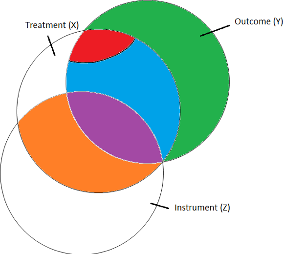
- The \(\color{green}{Green\, circle\, is\, the\, unexplained\, variation.}\)
- The \(\color{red}{Red\, circle\, is\, the\, correlated\, part\, of\, X\, with\, the\, error.}\)
- The \(\color{blue}{Blue\, circle\, is\, the\, uncorrelated\, part\, of\, X\, with\, the\, error.}\)
- The \(\color{orange}{Orange\, circle\, shows\, where\, X\, and\, Z\, are\, correlated.}\)
- The \(\color{purple}{Purple\, circle\, shows\, where\, X,\, Y,\, and\, Z\, are\, correlated.}\)
The fact that X overlaps with the error term and Y is the problem. So what we want to do is use the part of X that is not in the error term. But how do we separate that out?
This is where the instrumental variable comes into play. Notice the instrumental variable overlaps X, but not the error. Also, notice the instrumental variable z only overlaps Y when it is inside of X.
We can use the instrumental variable to capture the part of X that is not correlated with the error term. This will make it unbiased.
The drawback is that we lose variation in X. Typically, when we lose variation in X that means our standard errors tend to increase.
12.2 Education Example
\[ln(wage)= \beta_0+\beta_1*EDUC+\beta_2*EXP +\beta_3*EXP^2+...+u\]
What is \(u\)?
- Ability
- Motivation
- Everything Else that affects wage
Further, we can think of the Education as function. \[EDUC=f(GENDER,S-E, location, Ability, Motivation)\]
12.3 What influences Log wages?
\[\begin{align*} ln(wage) &=\beta_0+\beta_1*EDUC(X,Ability,Motivation)+\beta_2*EXP \\ &+\beta_3*EXP^2+...+u(Ability,Motivation)\end{align*}\]
Increased Ability is associated with increases in Education and \(u\).
What looks like an effect due to an increase in Education may be an increase in Ability.
The estimate of \(\beta_1\) picks up the effect of Education and the hidden effect of Ability.
An Exogenous Influence
\[ln(wage)=\beta_0+\beta_1*EDUC(Z,X,Ability,Motivation) \\ +\beta_2*EXP+\beta_3*EXP^2+...+u(Ability,Motivation)\]
A variable Z is associated with an increase in Education, but does not affect the error \(u\).
An effect due to an increase of Z on Education will only be an increase in Education. For changes in Z, we can estimate changes in log wages that are caused by education.
One example of a potential instrumental variable here is a surprise tuition voucher. Some people receive this vouchers and others do not. The voucher affects the cost of getting education, but are independent of the characteristics of the person receiving the voucher.
12.4 Instrumental Variables Regression
Three important threats to internal validity are:
- omitted variable bias from a variable that is correlated with X but is unobserved, so cannot be included in the regression;
- simultaneous causality bias (X causes Y, Y causes X);
- errors-in-variables bias or measurement error (X is measured with error)
Instrumental variables regression can eliminate bias when \(E(u|X) \ne 0\) by using an instrumental variable, Z
12.4.1 Examples of Omitted Variable Bias
Example 1: Income and Education
Suppose we want to study the relationship between income and happiness. We collect data from a sample of individuals and find a positive correlation between income and happiness, suggesting that higher income leads to higher levels of happiness. However, we omitted the variable “education” from the analysis. Education is likely to be related to both income and happiness. People with higher education tend to have higher incomes and may also experience higher levels of happiness due to job satisfaction, opportunities for personal growth, and better life choices. By not including education in the analysis, we introduce omitted variable bias, and the estimated effect of income on happiness may be inflated or deflated.
Example 2: Advertising and Sales
Consider a company that wants to determine the impact of advertising expenditure on product sales. They collect data on advertising spending and sales for a few months and find a positive correlation between advertising expenditure and sales. However, they forget to include the variable “seasonality” in their analysis. Seasonality refers to the influence of seasons or holidays on sales. During certain seasons (e.g., Christmas, summer vacation), both advertising spending and sales may increase due to increased consumer demand. By not accounting for seasonality, the estimated effect of advertising on sales could be biased and not accurately reflect the true causal relationship.
Example 3: Unemployment and Crime Rates
A researcher wants to study the relationship between unemployment rates and crime rates across different cities. They collect data from several cities and find a positive correlation between unemployment and crime rates, suggesting that higher unemployment leads to more crime. However, they omit the variable “poverty rate” from the analysis. Poverty is likely to be related to both unemployment and crime rates. High poverty rates can lead to both higher unemployment (fewer job opportunities) and higher crime rates (due to desperation and lack of resources). By not considering poverty rates, the estimated effect of unemployment on crime rates may be biased.
In all these examples, omitting a relevant variable results in omitted variable bias, leading to incorrect conclusions about the true relationship between the variables of interest. To address this bias, researchers should carefully select and include all relevant variables in their analysis to obtain more accurate and reliable results.
12.4.2 Examples of Simultaneity Bias
Example 1: Income and Consumption
Suppose we want to examine the relationship between income and consumption expenditure of households. On one hand, it is logical to assume that higher income leads to increased spending on consumption. However, the relationship can also work the other way around. Higher consumption can lead to higher income if, for instance, increased spending stimulates the economy and generates more income for individuals. In this case, the true relationship between income and consumption is simultaneous, and analyzing them in a standard linear regression model without addressing the simultaneity can lead to biased and misleading results.
Example 2: Education and Income
Consider a study that aims to explore the relationship between education level and income. It is commonly believed that higher education leads to better job opportunities and higher income. However, income can also influence education choices. Individuals with higher-income backgrounds might have better access to education resources and might pursue higher education more frequently. Thus, the relationship between education and income is simultaneous, and a standard regression analysis without accounting for simultaneity can produce biased estimates of the true relationship.
Example 3: Investment and Profitability
A company wants to assess the impact of investment in new technology on its profitability. On one hand, increased investment in technology might lead to improved efficiency and productivity, resulting in higher profitability. On the other hand, a more profitable company might have more resources available to invest in technology. Hence, the relationship between investment and profitability is simultaneous, and failing to address simultaneity in the analysis can lead to erroneous conclusions about the true causal relationship.
Example 4: Interest Rates and Investment
An economist wants to study the relationship between interest rates and investment levels in an economy. Lower interest rates might encourage borrowing and investment, while higher investment levels could stimulate economic growth and lead to lower interest rates due to increased demand for credit. In this case, the relationship between interest rates and investment is simultaneous, and not accounting for simultaneity in the analysis can result in biased estimates of the true effect of interest rates on investment.
12.4.3 Examples of Measurement Error
Example 1: Height and Weight Relationship
Suppose researchers are interested in studying the relationship between height and weight in a population. They collect data from a sample of individuals and measure their height and weight. However, due to measurement error, some height and weight values may be recorded incorrectly. For instance, the measuring instrument may not be calibrated correctly, or human errors might occur during data entry. As a result, the relationship between height and weight obtained from the data will be distorted due to the inaccuracies in the measurements.
Self-reported data tends to introduce both exogenous and endogenous measurement error. That is, measurement error that occurs because of random recall mistakes (exogenous) versus measurement error done to conceal/hide/lie endogenous.
Let’s look at height again for example of endogenous measurement error.
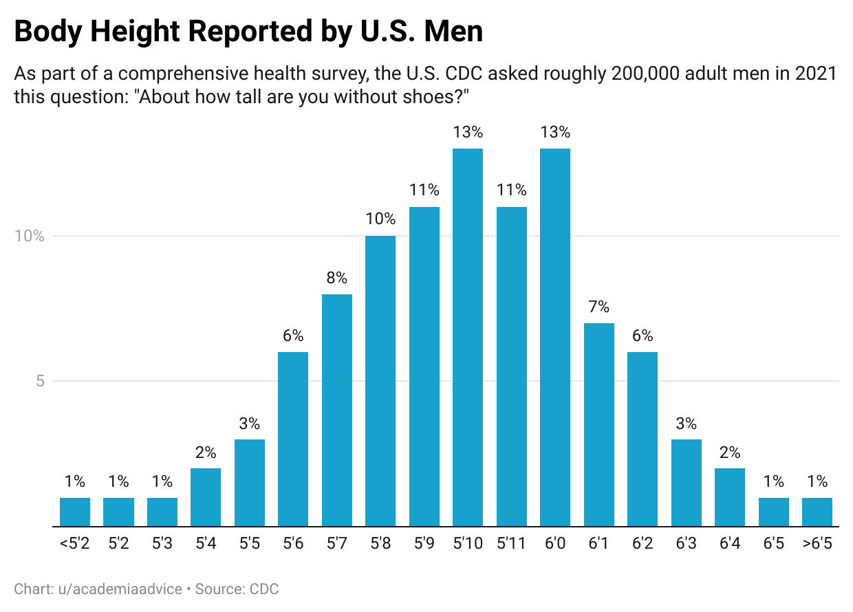
The histogram captures self-reported height among men. Notice, the histogram appears normally distributed until you get to 5’11”. You also see a pretty big drop off from 6’0” to 6’1”. This discrepancy seems suspicious as if people are lying about their height. 6’0” is a focal point here.
One reason that this could be occurring is due to self-esteem. Here is essentially the same graph, but now we include the percent of men who are “OK, with their height”. We do the same for women as well. You will see the 5’11” blip again among the men who were surveyed. You also notice the rapid increase in satisfaction with height 5’7” to 6’0”.
Example 2: Self-Reported Income and Spending Habits
A researcher wants to investigate the relationship between self-reported income and spending habits of individuals. They administer a survey asking respondents to report their income and their monthly expenditures. However, self-reported income and spending may not always be accurate due to various reasons. Respondents might overstate or understate their income or expenses for various personal or social reasons. This measurement error in income and spending data could lead to biased estimates of the relationship between income and spending habits.
Example 3: Test Scores and Job Performance
An organization is interested in understanding the relationship between test scores of job applicants and their subsequent job performance. They conduct pre-employment tests to assess the abilities of the applicants and then track their job performance over time. However, the test scores might not fully capture the applicants’ true abilities due to measurement error. Some individuals may have performed better or worse on the test than their actual abilities would suggest due to factors like test anxiety, distractions during the test, or unfamiliarity with the format. Consequently, the estimated relationship between test scores and job performance may be biased because of the measurement error in the test scores.
Example 4: Survey Responses on Sensitive Topics
In a study examining attitudes toward sensitive topics like substance abuse, mental health, or illegal activities, researchers conduct surveys to gather data. However, respondents may provide inaccurate or dishonest responses due to social desirability bias or fear of revealing sensitive information. As a result, the collected data may not reflect the true attitudes and behaviors of the population, leading to measurement error bias in the estimated relationships between variables.
In all these examples, measurement error bias arises from inaccuracies in the measurement of variables, which can lead to distorted and unreliable estimates of relationships between variables in statistical analysis. Researchers must be aware of potential measurement errors and take appropriate measures to minimize their impact on the results. Techniques like using multiple measurements, validation studies, or sophisticated statistical methods can help mitigate measurement error bias to some extent.
12.4.4 Measurement Error Bias in Linear Regression
Suppose we are interested in the regression equation \[Y=\beta_0 + \beta_1X+e\]
Suppose we do not get to observe \(Y\), but instead observe \(\widetilde{Y}=Y+u\) where the \(u\) is a random error that is independent of \(e\) with mean zero and standard deviation \(\sigma_u\).
When there is measurement error in the dependent variable. You will still receive unbiased estimates, but your standard error will be larger.
\[\widetilde{Y}=\beta_0 + \beta_1X+e \\ \hat{\beta}=\frac{cov(\widetilde{Y},X)}{Var(X)}=\frac{cov(Y+u,X)}{Var(X)} \\ = \frac{cov(Y,X)}{Var(X)}+\frac{cov(u,X)}{Var(X)} \\ =\frac{cov(Y,X)}{Var(X)}\] Since \(u\) is independent of X, the covariance of X and u is zero. The only thing that really changes is that the new regression error becomes \(e-u\) and the \(Var(e-u)=\sigma^2_e+\sigma^2_u\). So the variance of the regression error increases, which makes all standard errors larger.
The logit here is that there is now even more variation in Y when the measurement error is present than before.
However, if the bias is in the X’s, then we do get a biased result.
Suppose we do not get to observe \(X\), but instead observe \(\widetilde{X}=X+u\) where the \(u\) is a random error that is independent of \(e\) with mean zero and standard deviation \(\sigma_u\).
\[Y=\beta_0 + \beta_1\widetilde{X}+e \\ \hat{\beta}=\frac{cov(Y,\widetilde{X})}{Var(\widetilde{X})}=\frac{cov(Y,X+u)}{Var(\widetilde{X})} \\ = \frac{cov(Y,X)}{Var(\widetilde{X})}+\frac{cov(Y,u)}{Var(\widetilde{X})} \\ =\frac{cov(Y,X)}{Var(\widetilde{X})}=\frac{cov(Y,X)}{Var(\widetilde{X})}\frac{Var(X)}{Var(X)} \\ = \frac{cov(Y,X)}{Var(X)}\frac{Var(X)}{Var(\widetilde{X})} \\ = \frac{cov(Y,X)}{Var(X)}\frac{\sigma^2_X}{\sigma^2_X+\sigma^2_u} \] Notice, when we have measurement error in X, our estimate is too small. The fraction \(\frac{\sigma^2_X}{\sigma^2_X+\sigma^2_u}<1\) which makes our final estimate too small. The larger the variance is of the measurement error, the smaller the estimated coefficient becomes.
12.5 The IV Model
Let our population regression model be
\[Y_i = \beta_0 + \beta_1 X_i + u_i,~~i=1,\dots,n\]
and let the variable \(Z_i\) be an instrumental variable that isolates the part of \(X_i\) that is uncorrelated with \(u_i\).
Endogeneity and Exogeneity
- We define variables that are correlated with the error term as endogenous
- We define variables that are uncorrelated with the error term as exogenous
- Exogenous variables are those that are determined outside our model
- Endogenous variables are determined from within our model. For example, in the cause of simultaneous causality, both our dependent variable \(Y\) and the regressor \(X\) are endogenous.
12.6 Conditions for a Valid Instrument
- Instrument relevance condition: \(Corr(Z_i, X_i) \ne 0\)
- Instrument exogeneity condition: \(Corr(Z_i, u_i) = 0\)
The first condition simply says that the instrument, \(Z\), is correlated with the endogenous variable of interest, \(X\). So \(Z\) explains some of \(X\).
The second condition says that \(Z\) is independent of the error term, \(u\). This means that Z can explain X, but does so only with the uncorrelated portion of X.
12.7 The Two Stage Least Squares Estimator
If valid instrument, \(Z\), is available, we are able to estimate the coefficient \(\beta_1\) using two stage least squares (TSLS).
- decompose \(X\) into its two components to isolate the component that is uncorrelated with the error terms. \[X_i = \underbrace{\pi_0 + \pi_1 Z_i}_{\text{uncorrelated component}} + v_i\]Since we don’t observe \(\pi_0\) and \(\pi_1\) we need to estimate them using OLS \[\hat{X}_i = \hat{\pi}_0 + \hat{\pi}_1 Z_i\]
Then, we use this uncorrelated component to estimate \(\beta_1\): we regress \(Y_i\) on \(\hat{X}_i\) using OLS to estimate \(\beta_0^{TSLS}\) and \(\beta_1^{TSLS}\).
Example: Philip Wright’s Problem
Suppose we wanted to estimate the price elasticity in the log-log model
\[\ln(Q_i^{butter}) = \beta_0 + \beta_1 \ln(P_i^{butter}) + u_i\]
if we had a sample of \(n\) observations of quantity demanded and the equilibrium price, we can run an OLS estimation to estimate the elasticity coefficient \(\beta_1\).
Supply and Demand
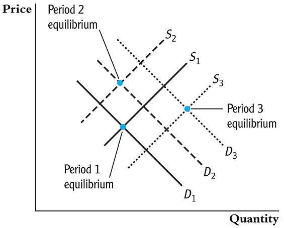
However, there is one big problem. We do not get to observed the supply and demand curves. Instead, we just observed the equilibrium points (where the lines cross).
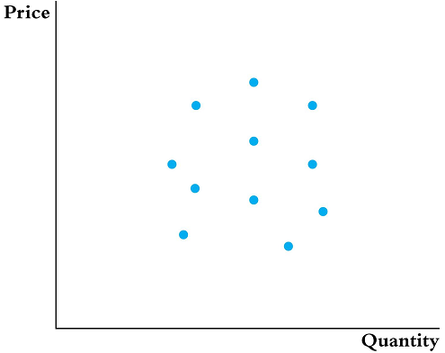 So how do you know you are estimating the demand curve or the supply curve?
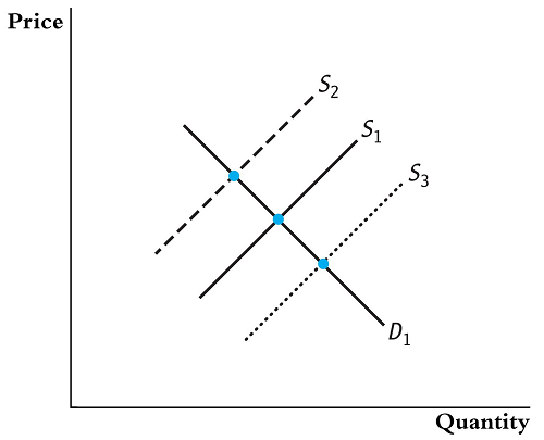
The secret is hidden back in your ECON 101 books. You need to think of things that shift the supply curve, but do not effect the demand curve.
We can use the supply shifters as instrumental variables to map out the demand curve.
Supply curve shifters are factors that can cause the supply curve for a particular good or service to shift either to the right (increase in supply) or to the left (decrease in supply). These shifts occur independently of changes in the price of the product and are influenced by various factors that affect the quantity of the product that suppliers are willing and able to offer at any given price level.
The main supply curve shifters include:
Input Prices: Changes in the prices of inputs used to produce the good or service can directly impact the cost of production. If input prices increase, the production becomes more expensive, leading to a decrease in supply, shifting the supply curve to the left. Conversely, if input prices decrease, the production cost decreases, leading to an increase in supply and shifting the supply curve to the right.
Technological Advancements: Improvements in technology and production processes can lead to increased efficiency and lower production costs. As a result, suppliers can produce more output at any given price level, leading to an increase in supply and shifting the supply curve to the right.
Number of Suppliers: If the number of producers or suppliers in the market increases, overall supply can increase. More suppliers mean more goods or services available in the market, leading to a rightward shift of the supply curve.
Expectations: If suppliers anticipate future changes in market conditions, they might adjust their production levels accordingly. For example, if suppliers expect higher prices in the future, they might reduce supply now to take advantage of those higher prices later. Conversely, if they anticipate lower prices in the future, they might increase supply in the present, shifting the supply curve accordingly.
Government Policies and Regulations: Government actions, such as taxes, subsidies, or regulations, can directly impact production costs or market conditions for suppliers. For instance, a subsidy to producers can reduce their costs and encourage an increase in supply, shifting the curve to the right. On the other hand, increased regulations might lead to higher compliance costs, reducing supply and shifting the curve to the left.
Natural Disasters and Weather Conditions: Natural disasters or adverse weather conditions can disrupt production processes and reduce the availability of inputs, leading to a decrease in supply and shifting the supply curve to the left.
Changes in Prices of Related Goods: If a producer can switch between producing different goods, changes in the prices of related goods can influence the willingness to supply a specific product. For example, if the price of an alternative product increases, suppliers might shift their focus to producing that alternative good, leading to a decrease in supply for the original product and shifting the supply curve to the left.
Understanding supply curve shifters is essential for economists, businesses, and policymakers to analyze and predict changes in market conditions and make informed decisions about resource allocation, pricing, and supply chain management.
Likewise, we can use demand shifters as instrumental variables to map out the supply curve.
Demand curve shifters are factors that can cause the demand curve for a particular good or service to shift either to the right (increase in demand) or to the left (decrease in demand). These shifts occur independently of changes in the price of the product and are influenced by various factors that affect the quantity of the product that consumers are willing and able to buy at any given price level.
The main demand curve shifters include:
Income: Changes in consumers’ income levels can significantly impact their purchasing power. For normal goods, which are goods for which demand increases as income increases, a rise in income will lead to an increase in demand, shifting the demand curve to the right. For inferior goods, which are goods for which demand decreases as income increases, a rise in income will lead to a decrease in demand, shifting the demand curve to the left.
Prices of Related Goods: The prices of related goods can affect the demand for a particular product. There are two types of related goods:
Substitutes: If the price of a substitute good (a product that can be used in place of the original product) decreases, the demand for the original product may decrease as consumers switch to the cheaper substitute. This leads to a decrease in demand for the original product and shifts its demand curve to the left.
Complements: If the price of a complementary good (a product that is often consumed together with the original product) decreases, the demand for the original product may increase as it becomes more attractive to consumers when paired with the cheaper complement. This leads to an increase in demand for the original product and shifts its demand curve to the right.
Tastes and Preferences: Changes in consumer preferences or tastes can lead to shifts in demand. If a product becomes more fashionable or desirable, its demand will increase, shifting the demand curve to the right. Conversely, if a product falls out of favor, its demand will decrease, shifting the demand curve to the left.
Population and Demographics: An increase in population or changes in demographic factors can affect the overall demand for certain goods and services. For example, a growing population in a region may lead to increased demand for housing, transportation, and other essential goods, shifting the demand curve to the right.
Expectations: Consumer expectations about future prices, income levels, or economic conditions can influence their current buying behavior. If consumers anticipate higher prices or incomes in the future, they may increase their current demand, shifting the demand curve to the right. Conversely, if they expect lower prices or incomes, they may decrease their current demand, shifting the demand curve to the left.
Government Policies: Government policies, such as taxes, subsidies, or regulations, can impact consumer behavior and influence demand. For example, a tax break on a particular product may increase its demand, shifting the demand curve to the right.
Understanding demand curve shifters is crucial for businesses, economists, and policymakers to analyze and predict changes in market conditions and make informed decisions about pricing, production, and marketing strategies.
12.9 Example: Estimating the Effect on Test Scores of Class Size
- Consider the estimation undertaken before using data from 420 California school districts
- A variety of regressors were added to the regression specification to address possible OVB.
- However, there are still some possible factors that are omitted: teacher quality and opportunities outside school.
- A possible hypothetical instrument: an earthquake causes closure of some schools until repairs are completed. Students are then expected to attend classes in neighboring schools unaffected by the earthquake causing an increase in their class sizes.
12.10 The Sampling Distribution of the TSLS Estimator
- The exact distribution of the TSLS estimator is complicated in small samples.
- But in large samples it approaches a normal distribution.
- Using a single regressor the calculation of the TSLS is simple \[\hat{\beta}_1^{TSLS} = \frac{s_{ZY}}{s_{ZX}}\]
This can be shown because
\[\begin{align*} Cov(Z_i, Y_i) &= Cov[Z_i, (\beta_0 + \beta_1 X_i + u_i)]\\ &= \beta_1 Cov(Z_i, X_i) + Cov(Z_i, u_i) \end{align*}\]
And since \(Cov(Z_i, u_i) = 0\) and \(Cov(Z_i, X_i) \ne 0\)
\[\beta_1 = \frac{Cov(Z_i, Y_i)}{Cov(Z_i, X_i)}\] If Z and X are not highly correlated with one another, then the denominator will be close to zero. This means very small changes in the numerator could lead to very large changes in the estimated \(\beta_{IV}\). We want that denominator to be stable so we need X and Z to be highly correlated.
Since \[\begin{align*} s_{ZY} &\overset{p}{\longrightarrow} Cov(Z_i, Y_i) \\ s_{ZX} &\overset{p}{\longrightarrow} Cov(Z_i, X_i) \end{align*}\]
therefore
\[\hat{\beta}_1^{TSLS} = \frac{s_{ZY}}{s_{ZX}} \overset{p}{\longrightarrow} \frac{Cov(Z_i, Y_i)}{Cov(Z_i, X_i)} = \beta_1\]
12.11 Application to the Demand for Cigarettes
- Consider the question of imposing a tax on cigarettes in order to reduce illness and deaths from smoking-in addition to other negative externalities on society.
- If the elasticity of demand is responsive to changes in cigarette prices, then it would be easy to impose a policy to reduce smoking by any desired proportion.
- We need to estimate this elasticity, but we cannot rely on data of demand and prices
- We need to use an instrumental variable.
We have cross-sectional data from 48 US states in 1995 with the variables
- \(SalesTax_i\): Which we use as an instrument.
- \(Q_i^{cigarettes}\): Cigarette consumption: number of packs sold/capita in state \(i\)
- \(P_i^{cigarettes}\): Average real price/pack including all taxes
Before we can carry out TSLS estimation we must investigate the relevance of our instrument.
- First, instrument relevance: since higher sales taxes would lead to higher cigarette prices this condition is plausibly satisfied.
- Second, instrument exogeneity: since sales taxes are set driven by questions of public finance and politics, and not questions of cigarette consumption, this condition is also plausibly satisfied.
Statistical software conceals the various steps needed for IV regression, but it can be useful to demonstrate the steps here
The first state regression yields \[\begin{alignat*}{2} \widehat{\ln(P_i^{cigarettes})} = &4.63 + &&~0.031 SalesTax_i \\ &(0.03) &&~(0.005) \end{alignat*}\]
with \(R^2 = 0.47\).
12.11.1 Data
cig.data=CigarettesSW
cig.data$packpc=cig.data$pack
cig.data$ravgprs <- cig.data$price/cig.data$cpi # real average price
cig.data$rtax <- cig.data$tax/cig.data$cpi # real average cig tax
cig.data$rtaxs <- cig.data$taxs/cig.data$cpi # real average total tax
cig.data$rtaxso <- cig.data$rtaxs - cig.data$rtax # instrument
The first stage regression
first.stage.res <- lm(log(ravgprs) ~ rtaxso, data=cig.data, subset=(year == 1995))
coeftest(first.stage.res, vcov.=vcovHAC(first.stage.res))
##
## t test of coefficients:
##
## Estimate Std. Error t value Pr(>|t|)
## (Intercept) 4.6165463 0.0285440 161.7343 < 2.2e-16 ***
## rtaxso 0.0307289 0.0048623 6.3198 9.588e-08 ***
## ---
## Signif. codes: 0 '***' 0.001 '**' 0.01 '*' 0.05 '.' 0.1 ' ' 1In the second stage, \(\ln(Q_i^{cigarettes})\) is regressed on \(\widehat{\ln(P_i^{cigarettes})}\) \[\begin{alignat*}{3} \widehat{\ln(Q_i^{cigarettes})} = &9.72 - &&~1.08 \widehat{\ln(P_i^{cigarettes})} \\ &(1.53) &&~(0.32) \end{alignat*}\]
IV regression in R
library(AER)
iv.res <- ivreg(log(packpc) ~ log(ravgprs) | rtaxso, data=cig.data, subset=(year == 1995))
coeftest(iv.res, vcov.=vcovHAC(iv.res))
##
## t test of coefficients:
##
## Estimate Std. Error t value Pr(>|t|)
## (Intercept) 9.71988 1.52719 6.3646 8.211e-08 ***
## log(ravgprs) -1.08359 0.31869 -3.4002 0.001401 **
## ---
## Signif. codes: 0 '***' 0.001 '**' 0.01 '*' 0.05 '.' 0.1 ' ' 1This is a strong relationship between prices and demand.
But perhaps our assumption of exogeneity might not be very valid.
Consider income: states with higher income might not need to rely on taxes for revenue and there is presumably an effect of income on consumption of cigarettes.
12.12 The General IV Regression Model
Variables of the General IV Regression Model
\[Y_i = \beta_0 + \beta_1 X_{1i} + \cdots + \beta_k X_{ki} + \beta_{k+1} W_{1i} + \cdots + \beta_{k+r}W_{ri} + u_i\]
For \(i = 1,\dots,n\),
- dependent variable: \(Y_i\)
- endogenous regressors: \(X_{1i},\dots, X_{ki}\)
- included exogenous regressors: \(W_{1i},\dots\)
- instrumental variables: \(Z_{1i},\dots, Z_{mi}\)
Let \(m\) be the number of instruments and \(k\) be the number of endogenous regressors. The coefficients of this model are said to be
- exactly identified: if \(m = k\)
- overidentified: if \(m > k\)
- underidentified: if \(m < k\)
For an IV regression to be possible, we must have exact identification or overidentification.
Included Exogenous Variables and Control Variables in IV Regression
The variables in \(W\) can either be
- exogenous variables: in which case \(E[u_i|W_i] = 0\)
- control variables: which have no causal interpretation are used to ensure there is no correlation between the included and instrumental variables and the error terms.
For example, in the model
\[\ln(Q_i^{cigarettes}) = \beta_0 + \beta_1\ln(P_i^{cigarettes}) + u_i\]
we raised the possibility of having income has an omitted factor that would be correlated with sales tax. If we added income directly or a control for it we can remove this bias.
Let our model be \[Y_i = \beta_0 + \beta_1 X_{i} + \beta_{2} W_{1i} + \cdots + \beta_{1+r}W_{ri} + u_i\] The first stage (which is often called the reduced form equation for \(X\)) would be \[\begin{align*} X_i = &\pi_0 + \pi_1 Z_{1i} + \cdots + \pi_m Z_{mi}\\ {}+ &\pi_{m+1} W_{i1} + \cdots + \pi_{m+r}W_{ri} + v_i \end{align*}\] and from it we can estimate \(\hat{X}_1, \dots, \hat{X}_n\).
The second stage would then be \[Y_i = \beta_0 + \beta_1 \hat{X}_{i} + \beta_{2} W_{1i} + \cdots + \beta_{1+r}W_{ri} + u_i.\] If we have multiple endogenous regressors, \(X_{1i},\dots,X_{ki}\), we would repeat the first stage for each of the \(k\) regressors, and plug them in in the second stage.
12.13 Conditions for Valid Instruments in the General IV Model
- Instrument relevance: In general if \(\hat{X}_{1i}\) denotes the predicted value for \(X_{1i}\) using the instruments \(Z\), then \((\hat{X}_{1i},\dots,\hat{X}_{ki},W_{1i}, W_{ri},1)\) must not be perfectly multicollinear.
- Instrument exogeneity: \(Corr(Z_{1i},u_i) = 0, \dots, Corr(Z_{mi}, u_i) = 0\)
12.13.1 The IV Regression Assumptions
- IV.A.1: \(E[u_i|W_{1i}, \dots, W_{ri}] = 0\).
- IV.A.2: \((X_{1i},\dots,X_{ki},W_{1i},\dots,W_{ri}, Z_{1i}, \dots, Z_{mi}, Y_i)\) are i.i.d. draws from their joint distribution.
- IV.A.3: Large outliers are unlikely
- IV.A.4: Instruments satisfy the two conditions for being valid.
12.13.2 Application to the Demand for Cigarettes
As stated before, when we regressed quantity demanded on prices, using sales taxes as an instrument, we might have correlation with the error since state income might be correlated with sales taxes. So, now let’s add an exogenous variable for income
\[\begin{alignat*}{5} \widehat{\ln(Q_i^{cigarettes})} = &9.43 - &&1.14 \widehat{\ln(P_i^{cigarettes})} + &&0.21\ln(Inc_i) \\ &(1.26) &&(0.37) && (0.31) \end{alignat*}\]
cig.data$perinc <- cig.data$income/(cig.data$pop * cig.data$cpi)

iv.res.2 <- ivreg(log(packpc) ~ log(ravgprs) + log(perinc)
                  | rtaxso + log(perinc), data=cig.data,
                  subset=(year == 1995))
coeftest(iv.res.2, vcov.=vcovHAC(iv.res.2))
##
## t test of coefficients:
##
## Estimate Std. Error t value Pr(>|t|)
## (Intercept) 9.43066 1.25464 7.5166 1.757e-09 ***
## log(ravgprs) -1.14338 0.37064 -3.0848 0.003477 **
## log(perinc) 0.21452 0.31145 0.6888 0.494509
## ---
## Signif. codes: 0 '***' 0.001 '**' 0.01 '*' 0.05 '.' 0.1 ' ' 1Now instead of using only one instrument we can use two: \(SalesTax_i\) and \(CigTax_i\), so \(m = 2\), making this model overidentified.
\[\begin{alignat*}{5} \widehat{\ln(Q_i^{cigarettes})} = &9.89 - &&1.28 \widehat{\ln(P_i^{cigarettes})} + &&0.28\ln(Inc_i) \\ &(0.96) &&(0.25) &&(0.25) \end{alignat*}\]
iv.res.3 <- ivreg(log(packpc) ~ log(ravgprs) + log(perinc)
                  | rtaxso + rtax + log(perinc), data=cig.data,
                  subset=(year == 1995))
coeftest(iv.res.3, vcov.=vcovHAC(iv.res.3)) # For Robust Standard Errors
##
## t test of coefficients:
##
## Estimate Std. Error t value Pr(>|t|)
## (Intercept) 9.89496 0.96599 10.2434 2.435e-13 ***
## log(ravgprs) -1.27742 0.25299 -5.0493 7.805e-06 ***
## log(perinc) 0.28040 0.25461 1.1013 0.2766
## ---
## Signif. codes: 0 '***' 0.001 '**' 0.01 '*' 0.05 '.' 0.1 ' ' 112.14 Checking Instrument Validity
- How do you know you have good instruments?
12.14.0.1 Assumption #1: Instrument Relevance
- The relevance of an instrument (the more the variation in \(X\) is explained by the instrument) plays the same role as sample size: it produces more accurate estimators.
- Instruments that do not explain a lot of the variation in \(X\) are called weak instruments. For example, distance of the state from cigarette manufacturing.
12.14.1 Why Weak Instruments are a Problem?
If instruments are weak, it is like having a very small sample size: the approximation of the estimator’s distribution to the normal distribution is very poor.
Recall that with a single regressor and instrument \[\hat{\beta}_1^{TSLS} = \frac{s_{ZY}}{s_{ZX}} \overset{p}{\longrightarrow} \frac{Cov(Z_i, Y_i)}{Cov(Z_i, X_i)} = \beta_1\]
Suppose that the instrument is completely irrelevant so that \(Cov(Z_i, X_i) = 0\), then \[s_{ZX} \overset{p}{\longrightarrow} Cov(Z_i, X_i) = 0\] Causing the denominator of \(Cov(Z_i,Y_i)/Cov(Z_i,X_i)\) to be zero, which makes the distribution of \(\beta_1^{TSLS}\) not normal.
A similar problem would be encountered with instruments that are not completely irrelevant but are weak.
To check for weak instruments, compute the \(F\)-statistic testing the hypothesis that the coefficients on all the instruments are zero in the first stage.
A rule of thumb is not to worry about weak instruments if the first-stage \(F\)-statistic is greater than 10.
If the model is overidentified and we have both weak and strong instruments, it is best to drop the weak instruments
However, if the model is exactly identified, it is not possible to drop any instruments.
In this case, we should try find stronger instruments (not a very easy task) or use the weak instruments with other methods than TSLS that are less sensitive to weak instruments.
Suppose that the instrument is completely irrelevant so that \(Cov(Z_i, X_i) = 0\), then \[s_{ZX} \overset{p}{\longrightarrow} Cov(Z_i, X_i) = 0\]
Causing the denominator of \(Cov(Z_i,Y_i)/Cov(Z_i,X_i)\) to be zero, which makes the distribution of \(\beta_1^{TSLS}\) not normal.
A similar problem would be encountered with instruments that are not completely irrelevant but are weak.
To check for weak instruments, compute the \(F\)-statistic testing the hypothesis that the coefficients on all the instruments are zero in the first stage.
A rule of thumb is not to worry about weak instruments if the first-stage \(F\)-statistic is greater than 10.
12.14.2 Assumption #2: Instrument Exogeneity
If the instruments are not exogenous then TSLS estimators will suffer from inconsistency.
Can Exogeneity be Statistically Tested?
- If the model is exactly identified we cannot test for exogeneity
- If the model is overidentified it is possible to test the hypothesis that the “extra’’ instruments are exogenous under the assumption that there are enough valid instruments to identify the coefficients of interest (test of overidentified restrictions).
12.14.3 The Overidentifying Restrictions Test (The J-Statistic)
- Suppose you have a model with one endogenous regressor and two instruments
- We can test for exogeneity by running two IV regressions once with each of the instruments
- If they are both valid, we should expect our estimates to be close, otherwise we should be suspicious of the validity one or both of the instruments.
We can test for exogeneity using the \(J\)-statistic. We do this by estimating the following regression
\[\begin{align*} \hat{u}_i^{TSLS} = &\delta_0 + \delta_1 Z_{1i} + \cdots + \delta_m Z_{mi}\\ {}+ &\delta_{m+1} W_{1i} + \cdots + \delta_{m+r} W_{ri} + e_i \end{align*}\]
and using an \(F\)-test for \(\delta_1 = \cdots = \delta_m = 0\)
12.15 Overidentification Test witin the Application to the Demand for Cigarettes
In our previous TSLS we used two instruments: \(SalesTax_i\) and \(CigTax_i\), and one exogenous regressor: state income.
There are still concerns about the exogeneity of \(CigTax_i\): there could be state specific characteristics that influence both cigarette taxes and cigarette consumption.
Luckily, we have panel data so we can eliminate state fixed effects.
To simplify matters we will focus on the differences between 1985 and 1995.
We regress \([\ln(Q_{i,1995}^{cigarettes}) - \ln(Q_{i,1985}^{cigarettes})]\) on \([\ln(P_{i,1995}^{cigarettes}) - \ln(P_{i,1985}^{cigarettes})]\) and \([\ln(Inc_{i,1995}) - \ln(Inc_{i,1985})]\)
- We use as instruments \([SalexTax_{i,1995} - SalesTax_{i,1985}]\) and \([CigTax_{i,1995} - CigTax_{i,1985}]\)
We are actually going to run a state fixed effects regression using all the data.
panel.iv.res.1 <- plm(log(packpc) ~ log(ravgprs) + log(perinc)
                      | rtaxso + log(perinc), data=cig.data,
                      method="within", effect="individual",
                      index=c("state", "year"))
coeftest(panel.iv.res.1, vcov.=vcovHC(panel.iv.res.1))
##
## t test of coefficients:
##
## Estimate Std. Error t value Pr(>|t|)
## log(ravgprs) -1.072460 0.168316 -6.3717 8.011e-08 ***
## log(perinc) -0.079004 0.254929 -0.3099 0.758
## ---
## Signif. codes: 0 '***' 0.001 '**' 0.01 '*' 0.05 '.' 0.1 ' ' 1First Stage \(F\)-test
panel.1st.stage.res.1 <- lm(log(ravgprs) ~ rtaxso, data=cig.data)
lht(panel.1st.stage.res.1, "rtaxso = 0", vcov=vcovHAC)
## Linear hypothesis test
##
## Hypothesis:
## rtaxso = 0
##
## Model 1: restricted model
## Model 2: log(ravgprs) ~ rtaxso
##
## Note: Coefficient covariance matrix supplied.
##
## Res.Df Df F Pr(>F)
## 1 95
## 2 94 1 112.64 < 2.2e-16 ***
## ---
## Signif. codes: 0 '***' 0.001 '**' 0.01 '*' 0.05 '.' 0.1 ' ' 1Difference IV
panel.iv.res.2 <- plm(log(packpc) ~ log(ravgprs) + log(perinc)
                      | rtax + log(perinc), data=cig.data,
                      method="within", effect="individual",
                      index=c("state", "year"))
coeftest(panel.iv.res.2, vcov.=vcovHC(panel.iv.res.2))
##
## t test of coefficients:
##
## Estimate Std. Error t value Pr(>|t|)
## log(ravgprs) -1.36316 0.16975 -8.0303 2.668e-10 ***
## log(perinc) 0.34247 0.24179 1.4164 0.1634
## ---
## Signif. codes: 0 '***' 0.001 '**' 0.01 '*' 0.05 '.' 0.1 ' ' 1First Stage \(F\)-test
panel.1st.stage.res.2 <- lm(log(ravgprs) ~ rtax, data=cig.data)
lht(panel.1st.stage.res.2, "rtax = 0", vcov=vcovHAC)
## Linear hypothesis test
##
## Hypothesis:
## rtax = 0
##
## Model 1: restricted model
## Model 2: log(ravgprs) ~ rtax
##
## Note: Coefficient covariance matrix supplied.
##
## Res.Df Df F Pr(>F)
## 1 95
## 2 94 1 302.12 < 2.2e-16 ***
## ---
## Signif. codes: 0 '***' 0.001 '**' 0.01 '*' 0.05 '.' 0.1 ' ' 1This time we include both instruments
panel.iv.res.3 <- plm(log(packpc) ~ log(ravgprs)
                      + log(perinc) | rtaxso + rtax + log(perinc),
                      data=cig.data, method="within", effect="individual",
                      index=c("state", "year"))
coeftest(panel.iv.res.3, vcov.=vcovHC(panel.iv.res.3))
##
## t test of coefficients:
##
## Estimate Std. Error t value Pr(>|t|)
## log(ravgprs) -1.26750 0.15872 -7.9858 3.103e-10 ***
## log(perinc) 0.20378 0.23261 0.8761 0.3855
## ---
## Signif. codes: 0 '***' 0.001 '**' 0.01 '*' 0.05 '.' 0.1 ' ' 1First Stage \(F\)-test
panel.1st.stage.res.3 <- lm(log(ravgprs) ~ rtaxso + rtax, data=cig.data)
lht(panel.1st.stage.res.3, c("rtaxso = 0", "rtax = 0"), vcov=vcovHAC)
## Linear hypothesis test
##
## Hypothesis:
## rtaxso = 0
## rtax = 0
##
## Model 1: restricted model
## Model 2: log(ravgprs) ~ rtaxso + rtax
##
## Note: Coefficient covariance matrix supplied.
##
## Res.Df Df F Pr(>F)
## 1 95
## 2 93 2 165.2 < 2.2e-16 ***
## ---
## Signif. codes: 0 '***' 0.001 '**' 0.01 '*' 0.05 '.' 0.1 ' ' 1Hansen J-test
j.test.reg <- lm(panel.iv.res.3$residuals ~ rtaxso + rtax + log(perinc), data=cig.data)
lht(j.test.reg, c("rtaxso = 0", "rtax = 0"), vcov.=vcovHAC)
## Linear hypothesis test
##
## Hypothesis:
## rtaxso = 0
## rtax = 0
##
## Model 1: restricted model
## Model 2: panel.iv.res.3$residuals ~ rtaxso + rtax + log(perinc)
##
## Note: Coefficient covariance matrix supplied.
##
## Res.Df Df F Pr(>F)
## 1 94
## 2 92 2 0.0012 0.998812.16 References
J. Angrist, “Lifetime Earnings and the Vietnam Era Draft Lottery: Evidence from Social Security Administrative Records,” American Economic Review, June 1990. 5
J. Angrist and A. Krueger, “Does Compulsory School Attendance Affect Schooling and Earnings?”, Quarterly Journal of Economics 106, November 1991.
J. Angrist, et al., “Who benefits from KIPP?”, J. of Policy Analysis and Management, Fall 2012.
J. Angrist, V. Lavy, and A. Schlosser, “Multiple Experiments for the Quantity and Quality of Children”, Journal of Labor Economics 28, October 2010.