Chapter 10 Causal Inference
10.1 Predictive vs Prescriptive
In Data Analytics there are often three types of answers
- Descriptive - Aim is to aggregate and describe your current data (a snapshot)
- Tables, Charts, Maps, Tableau
- Predictive - Aim is to predict the dependent variable. How will it change in the near future?
- Machine Learning
- Time Series Forecast
- Prescriptive - Aim is to explain the dependent variable. What is the effect of your advertising campaign? Why are workers leaving your firm?
- What this course is about!
Linear Regression Models for Causal Inference
- Randomized Experiments
- Simple Linear Regression
- Multiple Regression
- Difference-in-Differences
- Instrumental Variables
- Regression Discontinuity
Two Types of Causal Questions
Two types of causal questions (Gelman and Imbens 2013):
- Reverse causal inference: search for causes of effects (Why?).
- Why does the United States perform so poorly in Math standardized exams?
- Forward causal questions: estimation of effects of causes (What if …?).
- Does teacher’s IQ affect students performance? Class size?
Causal effects
We are motivated by why questions but, when conducting our analysis, we tend to proceed by addressing what if questions.
Examples:
- How does taking this course affect your earnings in 3-years?
- Note that this is different from a predictive question: “What will be the earnings of students taking this course?”
- If Uber increases prices, how would it affect demand?
- Does the death penalty decrease crime rates?
- Would it be profitable for a firm to allow employees to work from home? (Yahoo 2013)
- Are employees more satisfied if they are informed about the salaries of their colleagues? (Card, Mas, Moretti and Saez 2012)
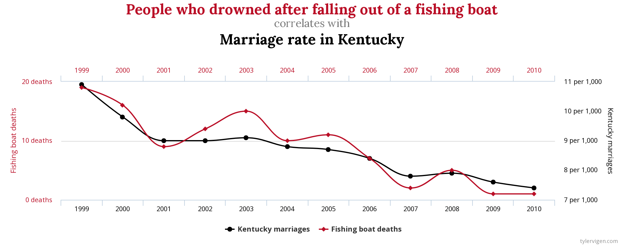
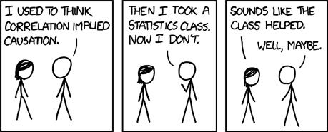
10.1.1 Correlation Does not Imply Causation
Two well known properties
- Correlation does not imply causation
- y can cause x even if x takes place before y
Less known property
- y can cause x
- x can cause y
- z can cause both x and y
10.1.2 Examples
Potentially confusing examples:
- Red cars are more likely to get involved in accidents
- People that sleep less tend to live longer
- Students living in households where there are more books tend to have higher GPA’s.
- Countries that eat more chocolate receive more Nobel prizes (Messerli 2012)
##
## Attaching package: 'kableExtra'
## The following object is masked from 'package:dplyr':
##
## group_rows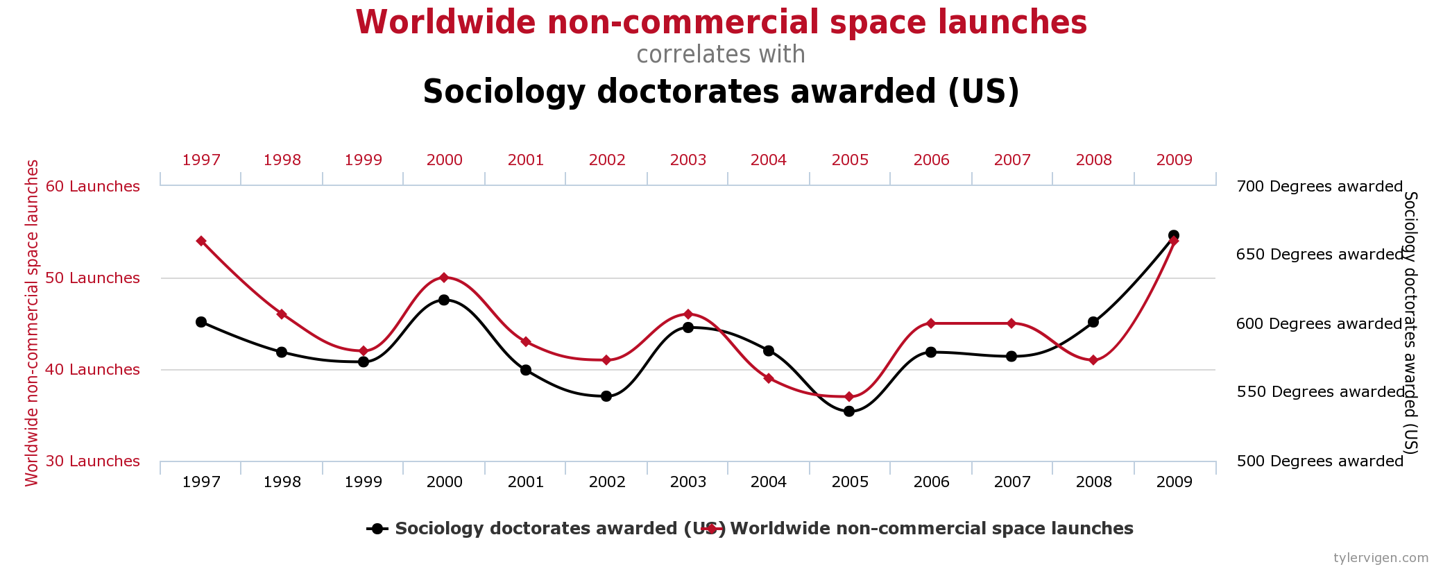
10.2 Randomized Experiments
10.2.1 How to Estimate Causal Effects
In the physical sciences:
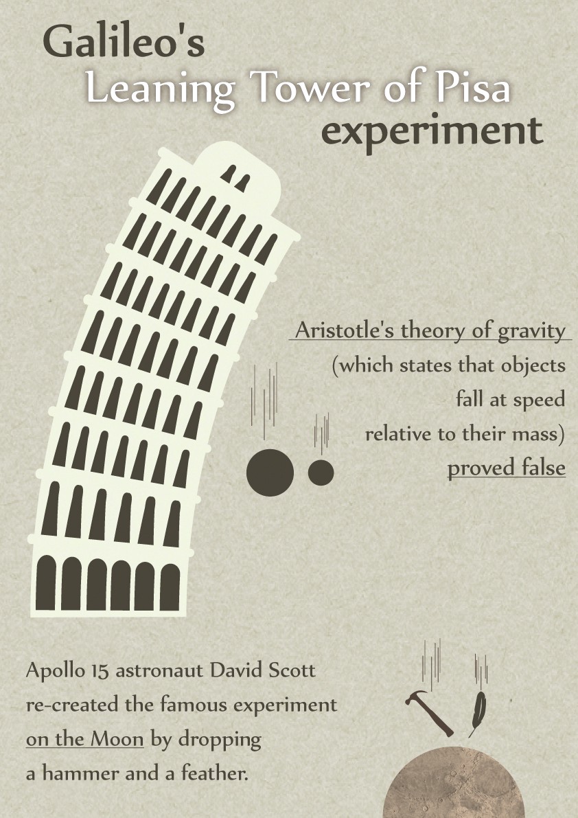
- Often, one can answer this type of question by running an experiment on a specific unit.
- Example: Galileo Galilei Leaning Tower of Pisa experiment
- Necessary conditions (ceteris paribus, other things being equal):
- Temporal stability: the response does not change if we change the moment when the treatment is applied.
- Causal transience: the response of one treatment is not affected by prior exposure of the unit to the other treatment.
- Unit homogeneity: homogeneity with respect to treatments and responses.
10.2.2 Leaning Tower of Pisa experiment
In the social sciences:
- None of these assumptions are plausible.
- We use a statistical solution: we estimate the average causal effect of the treatment over the population of units.
- Intuition: “All Other things being equal” conditions are likely to be satisfied on average across treated and non-treated if the treatment is randomly assigned.
10.2.3 Health Insurance Experiment
Suppose we are interested in the effect of health insurance on a person’s health
Let’s think of a treatment (getting insurance) for individual \(i\) as a binary random variable \(D_i = {0, 1}\) And potential outcomes (counterfactuals): \(Y_{0i}\), \(Y_{1i}\)
\(Y_{1i}\) = A measure of person \(i\)’s health given they have insurance \((D_i=1)\).
\(Y_{0i}\) = A measure of person \(i\)’s health given they do not have insurance \((D_i=0)\).
The individual treatment effects are \(Y_{1i} , Y_{0i}\)
Unfortunately, for person \(i\), we only observe \(Y_{1i}\) if \(D_i\) = 1 and \(Y_{0i}\) if \(D_i\) = 0
For any individual \(i\), we only observe \(Y_i=D_iY_{1i}+(1-D_i)Y_{0i}\)
That is, we only observe you in one state of the world. You either have insurance or you do not. This is a problem for us because there is no “counterfactual” version of you by which to compare.
What makes a good treatment effect estimate is not just if the treatment itself is effective, but it must also include a control group. A control group captures everything about you that would have occurred if you had not received the treatment.
In a supernatural (or highly advance sci-fi) world, there is a perfect twin of you. We give one of you the treatment and give the twin nothing, then compare outcomes. The only difference between the twins would be that one received treatment.
10.2.5 AVERAGE TREATMENT EFFECT
Returning to the problem, we cannot observe you as both having and not having insurance.
Solution is to look for the AVERAGE TREATMENT EFFECT (ATE)! \[E[Y_{1i}] - E[Y_{0i}]\] And a naive comparison of averages does not tell us what we want to know: \[E[Y_{1i}|D_{i} = 1] - E[Y_{0i}|D_{i} = 0]\] \[=\begin{array}{c}\underbrace{E[Y_{1i}|D_{i} = 1] - E[Y_{0i}|D_{i} = 1] }\\ ATE\end{array}+\begin{array}{c}\underbrace{E[Y_{0i}|D_{i} = 1] - E[Y_{0i}|D_{i} = 0] }\\ Sample \, Selection \, Bias\end{array}\]
Average treatment effect (ATE) and average treatment effect on the treated (ATT) need not to be the same and the distinction is sometimes important
They will be the same only if treatment is homogeneous across groups: \[E[Y_{1i} - Y_{0i}|D_i = 1] = E[Y_{1i} - Y_{0i}|D_i = 0] = E[Y_{1i} - Y_{0i}]\]
That is, the treatment is assigned randomly.
10.2.6 Random Assigment
We want to understand what would have happened to the treated in the absence of treatment and thus overcome the selection problem…
Solution : Random assignment
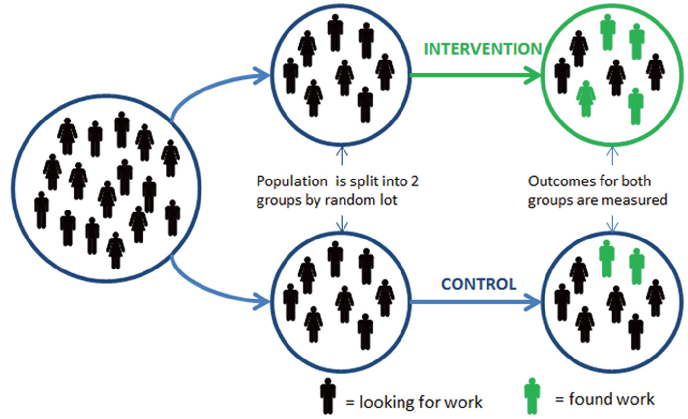
Random assignment makes \(D_i\) independent of potential outcomes, hence:
- the selection effect is zeroed out and
- the treatment effect on the treated is equal to the ATE.
10.2.7 Types of randomized experiments
A randomized experiment is designed and implemented consciously by social scientists. It entails conscious use of a treatment and control group with random assignment.
- Lab experiments
- The effect of feedback on relative performance (Azmat and Iriberri, 2012). Yes you work harder
- Field experiments (Lab-in-the-field)
- The effect of feedback on relative performance: (Bagues et al, work in progress) Yes Students work harder
- Natural experiments
- has a source of randomization that is as if randomly assigned, but not part of real experiment.
- Vietnam-era service effect on education and earnings (Flory, Leibbrandt and List 2010) Women Shy away from competitive work settings
10.2.8 Who uses Experiments in Business?
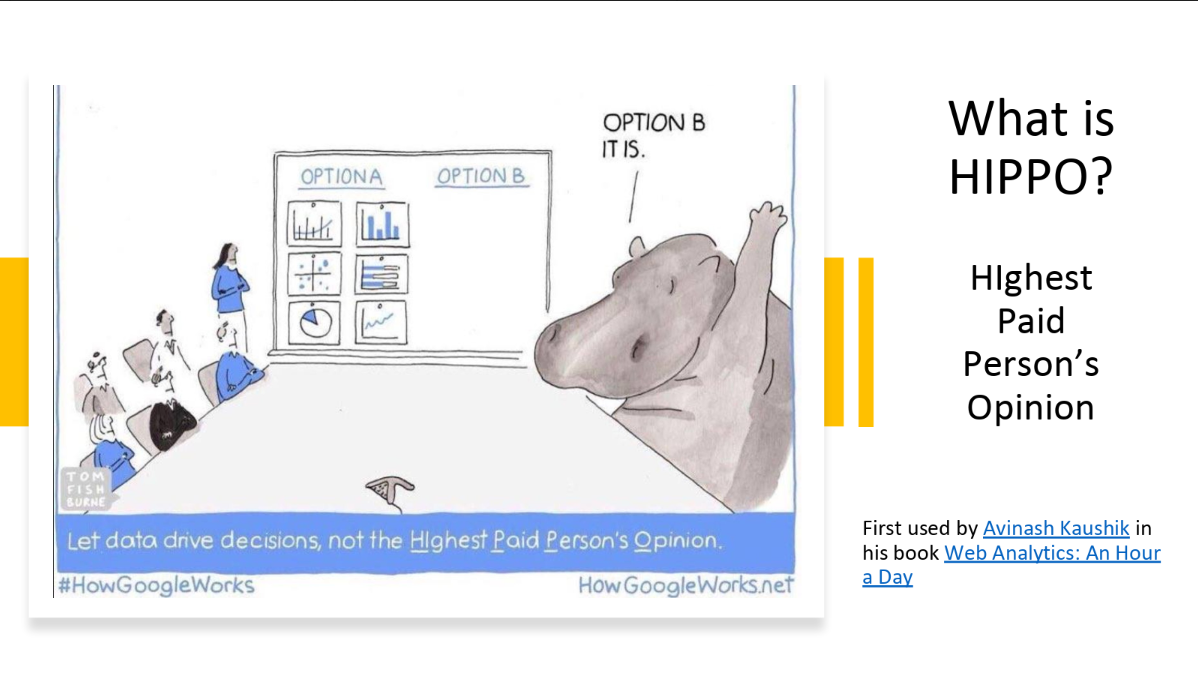
Tech Companies like Google, Facebook, and Amazon are positioned to use experiments.
They embraced the idea of “Data-Base Management” where the results of experiments were taken over the advice of HiPPO’s (Highest Paid Person’s Opinion)
THE A/B TEST: INSIDE THE TECHNOLOGY THAT’S CHANGING THE RULES OF BUSINESS, Wire Magazine 4 2012
In Praise of Data-Driven Management (AKA “Why You Should be Skeptical of HiPPO’s”)
10.2.9 Potential drawbacks of RCTs
Experiments provide a very transparent and simple empirical strategy. They solve the selection bias problem. However, there are a number of potential problems:
- Problems of implementation
- Compliance and attrition
- Cost, political issues (policy makers need to acknowledge ignorance),…
- Ethical issues
- Note that the ethical argument is not obvious when (i) the treatment cannot be applied to everybody (maybe due to some budget constraints) and (ii) the optimal assignment rule is unknown.
- Hawthorne effect
* People behave differently in experiments when they know they are being watched. Unfortunately, you may observe a treatment effect, but you are not sure if it is because of the intervention or because people are behaving differently because they know you are measuring their every move.
- The Illumination Experiment (Landsberger 1950, Levitt and List 2011)
- Audit study in France (Behaghel et al. 2015)

10.3 Rand Health Insurance Study

Conducted between 1974 and 1982
Randomly assigned thousands of non-elderly individuals and families to different insurance plan designs
Plans ranged from free care to $1,000 deductible (basically) with variations in between
Comparable deductible today is at least $4,000
Studied effects on health spending and health outcomes
| plantype | n | pct |
|---|---|---|
| Catastrophic | 759 | 0.1918120 |
| Deductible | 881 | 0.2226434 |
| Coinsurance | 1022 | 0.2582765 |
| Free | 1295 | 0.3272681 |
Patient Characteristics
| variable | Mean | Std. Dev. |
|---|---|---|
| Age | 32.36 | 12.92 |
| Pct. Black or Hispanic | 0.17 | 0.38 |
| Education | 12.10 | 2.88 |
| Pct. Female | 0.56 | 0.50 |
| General Health Index | 70.86 | 14.91 |
| Hospital | 0.12 | 0.32 |
| Income | 31603.21 | 18148.25 |
| Mental Health Index | 73.85 | 14.25 |
Patient Characteristics by Plan
| response | (Intercept) | Coinsurance | Deductible | Free |
|---|---|---|---|---|
| Age | 32.4 (0.485) | 0.966 (0.655) | 0.561 (0.676) | 0.435 (0.614) |
| Black/Hisp. | 0.172 (0.0199) | -0.0269 (0.025) | -0.0188 (0.0266) | -0.0281 (0.0245) |
| Educ. | 12.1 (0.14) | -0.0613 (0.186) | -0.157 (0.191) | -0.263 (0.183) |
| Female | 0.56 (0.0118) | -0.0247 (0.0153) | -0.0231 (0.016) | -0.0379 (0.015) |
| Gen. Health | 70.9 (0.694) | 0.211 (0.922) | -1.44 (0.952) | -1.31 (0.872) |
| Hospital | 0.115 (0.0117) | -0.00249 (0.0152) | 0.00449 (0.016) | 0.00117 (0.0146) |
| Income | 31,603 (1,073) | 970 (1,391) | -2,104 (1,386) | -976 (1,346) |
| Mental Health | 73.8 (0.619) | 1.19 (0.81) | -0.12 (0.822) | 0.89 (0.766) |
Notice, there is no statistical difference between patient demographics and treatment groups. This is the magic of random assignment. Therefore, any observed health differences between the treatment groups must be due to the treatment and not differences between the people in each group.
How do I know there isn’t a statistical difference? I am using a rule of thumb. I take the coefficient and divide it by the standard error (the value in parentheses). When the result is greater than 2 in absolute value terms, then that means it is like having a z-score > 2, which would make it significant at the 5 percent level.
Patient Health by Plan
| response | (Intercept) | Cost Sharing | Deductible | Free |
|---|---|---|---|---|
| face-to-face visits | 2.78 (0.178) | 0.481 (0.24) | 0.193 (0.247) | 1.66 (0.248) |
| Inpatient | 388 (44.9) | 92.5 (72.8) | 72.2 (68.6) | 116 (59.8) |
| Outpatient | 248 (14.8) | 59.8 (20.7) | 41.8 (20.8) | 169 (19.9) |
| Total Cost | 636 (54.5) | 152 (84.6) | 114 (79.1) | 285 (72.4) |
| Admissions | 0.0991 (0.00785) | 0.0023 (0.0108) | 0.0159 (0.0109) | 0.0288 (0.0105) |
This experiment is potentially the main reason the U.S. does not have universal health insurance today. What we learned from the experiment is that there does not seem to be a difference in physical health outcomes between groups, but there is a significant difference is usage of health care.
Check for yourself. Use the rule of thumb where we take the coefficient and divide it by the standard error. If it is greater than 2 in absolute value, then it is statistically significant. Which outcomes are statistically significant?
10.3.1 References
Experiments and Potential Outcomes MM, Chapter 1
J. Angrist, D. Lang, and P. Oreopoulos, “Incentives and Services for College Achievement: Evidence from a Randomized Trial”, American Economic Journal: Applied Economics, Jan. 2009.
A. Aron-Dine, L. Einav, and A. Finkelstein, “The RAND Health Insurance Experiment Three Decades Later”, J. of Economic Perspectives 27 (Winter 2013), 197-222.
R.H. Brook, et al., “Does Free Care Improve Adults’ Health?”, New England J. of Medicine 309 (Dec. 8, 1983), 1426-1434.
S. Taubman, et al., “Medicaid Increases Emergency-Department Use: Evidence from Oregon’s Health Insurance Experiment”, Science, Jan 2, 2014.