Chapter 15 Propensity Score Match
Propensity Score Matching (PSM) is a useful technique when using quasi-experimental or observational data (Austin, 2011; Rubin, 1983).
- It helps to create a counterfactual sample (control group) when random assignment is unavailable, unfeasible, or unethical.
- By using an index instead of specific covariates to match, PSM mitigates the curse of dimensionality associated with “exact match” techniques.
- Along with reducing the curse of dimensionality, this technique can be used in small samples where exact matches are infrequent or non-existent
15.1 Conceptual Model
The model \[y=z \gamma+X\beta+u\] Suppose you observe an outcome variable \(y\), a treatment variable \(z\), and a set of covariates in matrix \(X\).
If the standard assumption that \(E[Xu]=E[Zu]=0\) holds, then we can simply use OLS to estimate the treatment effect.
However, this assumption rarely holds in non-experimental settings. That is, the treatment assignment is endogenous (i.e. \(E[Zu]\ne0\))
The model \[y=z \gamma+X\beta+u\]
If we have an instrumental variable for \(z\), then we can still use IV to estimate the treatment effect.
Matching models become an option when
- No instrument is available
- We believe the covariates X are independent of the error term \(E[Xu]=0\).
We can use a two step process to help solve this problem.
Step 1. Use a probit or logit model to estimate \(Pr(z=1|X)\).
- This step allows us to estimate the likelihood that a person would receive treatment given their observable characteristics.
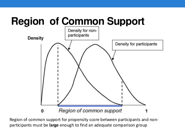
Step 2. Use the predict probability (propensity score) from Step 1 to match people in the treatment group with people in the control group that have very similar propensity scores.
- For example, if someone in the treatment group has a predicted probability of receiving treatment equal to 0.5, then we would like to match that person with someone who has a predicted probability close to 0.5, but who did not receive the treatment.
15.1.2 PSM Tips
Probit/Logit may not be the best method to construct the propensity score.
Machine Learning is particularly adapt to classification problems
Consider using a classification model like Boost to obtain propensity scores
15.1.3 Examples of Propensity Score problems
JobCorps is the largest free residential education and jobs programs. We may want to know the benefit of JobCorps on employment. However, individuals self-select into the JobCorps program.
Is there a wage penalty associated with smoking? People are not randomly assigned to be smokers. How can we estimate this affect?
Is there a benefit of attending private vs public school? Again, students are not randomly assigned to public or private schools
15.2 Other types of matching
Before we proceed with propensity score matching let’s consider two alternatives
- Exact Match: Here we match people in the treatment group with individuals in the control group that have identical observable characteristics (i.e. X’s).
- This method requires a lot of data.
- The assumption is that the unobserved portion of the individual is randomly distributed.
- We can average the outcome variable of the set of exact control matches and subtract that from the treatment outcome. The Law of Large numbers will give us an unbiased estimate as \(n \to \infty\).
Before we proceed with propensity score matching let’s consider two alternatives
- Mahalanobis Metric Matching: Relaxes the assumption of exact match. Instead, it calculates the distance between observation using a multidimensional distance metric.
- Requires less data than exact match.
- suffers from the curse of dimensionality.
- To reduce the curse of dimensionality remove X’s that are more randomly distributed between groups.
The distance formula is given by \[d(i,j)=(u-v) C^{-1} (u-v)^T\]
Let k be the number of covariates, then u is a row vector of covariate for person i (treatment) with the dimensions 1xk. Similarly, v is a row vector for person j (control). The matrix \(C^{-1}\) is the covariance matrix for the control group.
We match every person in the treatment with a person in the control group that has the smallest \(d(i,j)\)
It is possible that an individual from the control group who is selected as the match for a participant in the treatment group, is not close in a multidimensional space. The average distance between observations actually increases as we included more covariates (Gu & Rosenbaum, 1993; Stuart, 2010; Zhao, 2004).
In propensity score matching, we utilize the nearest-neighbor routine, which matches individuals in the treatment group with individuals in the control group who have the closest propensity score.
As in the Mahalanobis Metric, we need to take care that the distance is between matches is not to great. We can impose a caliper limit which states that \[||P_i-P_j||<\epsilon\]
where \(\epsilon=0.25*\sigma_p\) and \(\sigma_p\) is the standard deviation of the propensity score metric.
15.3 Advance Routines
You can combine PSM with Mahalanobis Metric by estimating the propensity scores and including the score as another covariate in the Mahalanobis Metric
Optimal Matching: This method uses propensity score match, but tries to minimize the total propensity score difference across all matches.
Full Matching: Is equivalent to optimal matching, but matches with replacement. That is, the same person can be used as a match in more than one pair.
15.4 Which Routine should I choose?
There are many choices and approaches to matching, including:
- Propensity score matching.
- Limited exact matching.
- Full matching.
- Nearest neighbor matching.
- Optimal/Genetic matching.
- Mahalanobis distance matching (for quantiative covariates only).
- Matching with and without replacement.
- One-to-one or one-to-many matching.
Which matching method should you use? Whichever one gives the best balance!
15.5 Propensity Match in R
15.5.1 National Supported Work
The National Supported Work (NSW) Demonstration was a federally and privately funded randomized experiment done in the 1970s to estimate the effects of a job training program for disadvantaged workers.
Participants were randomly selected to participate in the training program. Both groups were followed up to determine the effect of the training on wages.
Analysis of the mean differences (unbiased given randomization), was approximately $800.
Lalonde (1986) used data from the Panel Survey of Income Dynamics (PSID) and the Current Population Survey (CPS) to investigate whether non-experimental methods would result in similar results to the randomized experiment. He found results ranging from \(\$\) 700 to \(\$\) 16,000.
15.5.2 PSM: Dehejia and Wahba (1999)
Dehejia and Wahba (1999) later used propensity score matching to analyze the data.
- Comparison groups selected by Lalonde were very dissimilar to the treated group.
- By restricting the comparison group to those that were similar to the treated group, they could replicate the original NSW results.
- Using the CPS data, the range of treatment effect was between $1,559 to $1,681. The experimental results for the sample was approximately $1,800.
- The covariates available include: age, education level, high school degree, marital status, race, ethnicity, and earning sin 1974 and 1975.
- Outcome of interest is earnings in 1978.
15.5.3 Replication
Calculating the Propensity Score
library(MatchIt); data(lalonde)
library(cobalt)
lalonde$black <- ifelse(lalonde$race=="black",1,0)
lalonde$hispan <- ifelse(lalonde$race=="hispan",1,0)
lalonde.formu <- treat~age + educ + black+hispan + married + nodegree + re74 + re75
glm1 <- glm(lalonde.formu, family=binomial, data=lalonde)
stargazer::stargazer(glm1,type="text",single.row = TRUE)
##
## =============================================
## Dependent variable:
## ---------------------------
## treat
## ---------------------------------------------
## age 0.016 (0.014)
## educ 0.161** (0.065)
## black 3.065*** (0.287)
## hispan 0.984** (0.426)
## married -0.832*** (0.290)
## nodegree 0.707** (0.338)
## re74 -0.0001** (0.00003)
## re75 0.0001 (0.00005)
## Constant -4.729*** (1.017)
## ---------------------------------------------
## Observations 614
## Log Likelihood -243.922
## Akaike Inf. Crit. 505.844
## =============================================
## Note: *p<0.1; **p<0.05; ***p<0.01## Mahalanobis Metric Matching
m.mahal<-matchit(lalonde.formu,data=lalonde, replace=FALSE,distance="mahalanobis")
## Get matched Data
mahal.match<-match.data(m.mahal)
## PSM nearest neighbor
##m.nn<-matchit(lalonde.formu, data = lalonde, caliper=0.1, method ="nearest")
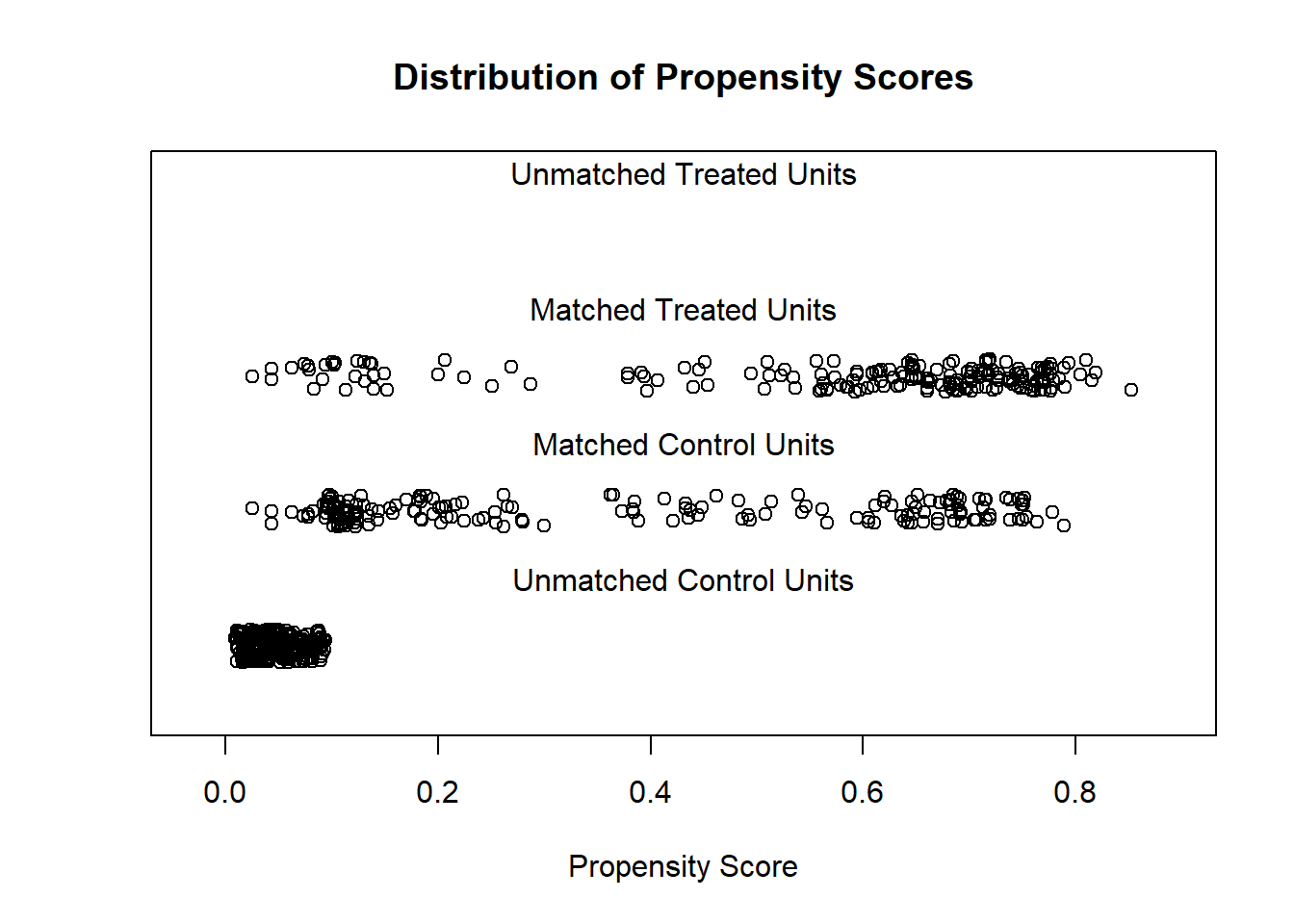
m.nn<-matchit(lalonde.formu, data = lalonde, ratio = 1, method ="nearest")
nn.match<-match.data(m.nn)library(RItools)
## Unconditional
xBalance(lalonde.formu, data = lalonde, report=c("chisquare.test"))## ---Overall Test---
## chisquare df p.value
## unstrat 238 8 6.17e-47## Nearest Neighbor
xBalance(lalonde.formu, data = as.data.frame(nn.match), report=c("chisquare.test"))## ---Overall Test---
## chisquare df p.value
## unstrat 61 8 2.99e-10Results
reg.1<-lm(re78~treat+age+educ+nodegree+re74+re75+married+black+hispan,data=lalonde)
reg.2<-lm(re78~treat+age+educ+nodegree+re74+re75+married+black+hispan,data=nn.match)
reg.3<-lm(re78~treat+age+educ+nodegree+re74+re75+married+black+hispan,data=mahal.match)
reg.2a<-lm(re78~treat,data=nn.match)
reg.3a<-lm(re78~treat,data=mahal.match)| Dependent variable: | |||||
| OLS | |||||
| (1) | (2) | (3) | (4) | (5) | |
| treat | 1,548.244** | 894.367 | 1,344.936* | 516.637 | 1,239.696 |
| (781.279) | (730.295) | (789.780) | (746.686) | (812.039) | |
| age | 12.978 | 7.804 | 15.112 | ||
| (32.489) | (42.915) | (45.720) | |||
| educ | 403.941** | 602.203*** | 533.042** | ||
| (158.906) | (224.070) | (243.621) | |||
| nodegree | 259.817 | 923.284 | -170.705 | ||
| (847.442) | (1,109.915) | (1,116.240) | |||
| re74 | 0.296*** | 0.026 | 0.071 | ||
| (0.058) | (0.103) | (0.098) | |||
| re75 | 0.232** | 0.221 | 0.272* | ||
| (0.105) | (0.160) | (0.155) | |||
| married | 406.621 | -158.255 | 653.748 | ||
| (695.472) | (986.307) | (984.773) | |||
| black | -1,240.644 | -469.434 | -1,158.148 | ||
| (768.764) | (1,009.928) | (906.948) | |||
| hispan | 498.897 | 1,064.045 | 1,120.562 | ||
| (941.943) | (1,300.198) | (1,676.953) | |||
| Constant | 66.515 | 5,454.776*** | -2,112.211 | 5,832.507*** | -453.365 |
| (2,436.746) | (516.396) | (3,511.770) | (527.987) | (3,546.028) | |
| Observations | 614 | 370 | 370 | 370 | 370 |
| R2 | 0.148 | 0.004 | 0.049 | 0.001 | 0.076 |
| Adjusted R2 | 0.135 | 0.001 | 0.025 | -0.001 | 0.053 |
| Residual Std. Error | 6,947.917 (df = 604) | 7,023.750 (df = 368) | 6,939.857 (df = 360) | 7,181.399 (df = 368) | 6,982.084 (df = 360) |
| F Statistic | 11.636*** (df = 9; 604) | 1.500 (df = 1; 368) | 2.054** (df = 9; 360) | 0.479 (df = 1; 368) | 3.313*** (df = 9; 360) |
| Note: | p<0.1; p<0.05; p<0.01 | ||||
Replication: Matched Dataset
#Order the matched dataset by pair ID
nn.match <- nn.match[order(nn.match$subclass),]

#Extract the outcomes for the treated and control
y1 <- nn.match$re78[nn.match$treat == 1]
y0 <- nn.match$re78[nn.match$treat == 0]

#Run the paired t-test
t.test(y1, y0, paired = TRUE)
##
## Paired t-test
##
## data: y1 and y0
## t = 1.2699, df = 184, p-value = 0.2057
## alternative hypothesis: true mean difference is not equal to 0
## 95 percent confidence interval:
## -495.1223 2283.8573
## sample estimates:
## mean difference
## 894.3675Replication: More on Balancing
## To identify the units, use first mouse button; to stop, use second.library(cobalt)
w.out1 <- WeightIt::weightit(
lalonde.formu,
data = lalonde, estimand = "ATE", method = "ps")
set.cobalt.options(binary = "std")
love.plot(w.out1)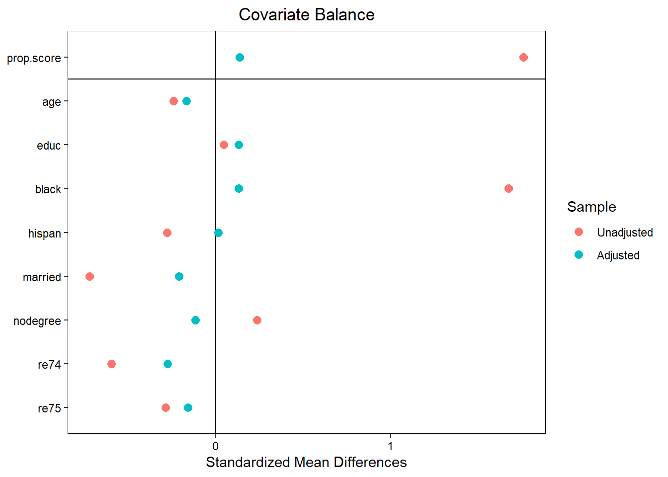
## Balance Measures
##             Type Diff.Un      M.Threshold.Un
## age      Contin. -0.2419 Not Balanced, >0.05
## educ     Contin.  0.0448     Balanced, <0.05
## black     Binary  1.6708 Not Balanced, >0.05
## hispan    Binary -0.2774 Not Balanced, >0.05
## married   Binary -0.7208 Not Balanced, >0.05
## nodegree  Binary  0.2355 Not Balanced, >0.05
## re74     Contin. -0.5958 Not Balanced, >0.05
## re75     Contin. -0.2870 Not Balanced, >0.05
##
## Balance tally for mean differences
##                     count
## Balanced, <0.05         1
## Not Balanced, >0.05     7
##
## Variable with the greatest mean difference
##  Variable Diff.Un      M.Threshold.Un
##     black  1.6708 Not Balanced, >0.05
##
## Sample sizes
##     Control Treated
## All     429     185
15.6 What else can we do with propensity scores?
Suppose you do not like the idea of throwing out data as we do with PSM
An alternative is to use weighted least squares where the propensity scores are the weights.
For treated individuals the weight is \[\frac{1}{Pr(treat=1)}\]
For control individuals the weight is \[\frac{1}{1-Pr(treat=1)}\]
15.6.2 PSM weights
| Dependent variable: | ||||||
| OLS | ||||||
| (1) | (2) | (3) | (4) | (5) | (6) | |
| treat | 1,548.244** | 894.367 | 1,344.936* | 516.637 | 1,239.696 | 712.743 |
| (781.279) | (730.295) | (789.780) | (746.686) | (812.039) | (552.508) | |
| age | 12.978 | 7.804 | 15.112 | 22.695 | ||
| (32.489) | (42.915) | (45.720) | (33.262) | |||
| educ | 403.941** | 602.203*** | 533.042** | 440.717*** | ||
| (158.906) | (224.070) | (243.621) | (167.840) | |||
| nodegree | 259.817 | 923.284 | -170.705 | 750.598 | ||
| (847.442) | (1,109.915) | (1,116.240) | (834.893) | |||
| re74 | 0.296*** | 0.026 | 0.071 | 0.197*** | ||
| (0.058) | (0.103) | (0.098) | (0.059) | |||
| re75 | 0.232** | 0.221 | 0.272* | 0.439*** | ||
| (0.105) | (0.160) | (0.155) | (0.108) | |||
| married | 406.621 | -158.255 | 653.748 | -433.395 | ||
| (695.472) | (986.307) | (984.773) | (654.412) | |||
| black | -1,240.644 | -469.434 | -1,158.148 | -958.637 | ||
| (768.764) | (1,009.928) | (906.948) | (610.182) | |||
| hispan | 498.897 | 1,064.045 | 1,120.562 | -351.844 | ||
| (941.943) | (1,300.198) | (1,676.953) | (910.924) | |||
| Constant | 66.515 | 5,454.776*** | -2,112.211 | 5,832.507*** | -453.365 | -444.515 |
| (2,436.746) | (516.396) | (3,511.770) | (527.987) | (3,546.028) | (2,529.555) | |
| Observations | 614 | 370 | 370 | 370 | 370 | 614 |
| R2 | 0.148 | 0.004 | 0.049 | 0.001 | 0.076 | 0.127 |
| Adjusted R2 | 0.135 | 0.001 | 0.025 | -0.001 | 0.053 | 0.114 |
| Residual Std. Error | 6,947.917 (df = 604) | 7,023.750 (df = 368) | 6,939.857 (df = 360) | 7,181.399 (df = 368) | 6,982.084 (df = 360) | 9,276.738 (df = 604) |
| F Statistic | 11.636*** (df = 9; 604) | 1.500 (df = 1; 368) | 2.054** (df = 9; 360) | 0.479 (df = 1; 368) | 3.313*** (df = 9; 360) | 9.788*** (df = 9; 604) |
| Note: | p<0.1; p<0.05; p<0.01 | |||||
Why are our results so off? Poor Balance
15.7 Summary
- PSM is useful when your binary treatment variable is endogenous, your explanatory variables are exogenous, and there a no available instruments.
- It is a solution to the “curse of dimensionality”
- It can be used to construct a better control group when running regressions
- Or on its own non-parametrically
- There is a tradeoff between balance and sample size
Extensions
- PSM can also be used to control for sample selection bias by using inverse propensity score matching weights in your regressions.
15.8 Business Analytics Example: Propensity Score Matching for Customer Retention
Propensity score matching is a statistical technique used in business analytics to assess the effectiveness of a treatment or intervention, such as a marketing campaign, on a particular outcome, such as customer retention. In this example, we’ll consider how a retail company uses propensity score matching to evaluate the impact of a loyalty program on customer retention.
Scenario:
Imagine a retail company that recently launched a loyalty program to encourage repeat purchases and improve customer retention. The company wants to determine whether the loyalty program is effective in increasing customer retention rates.
Data Collection:
The company collects data on a sample of customers who were part of the loyalty program (treatment group) and another sample of customers who were not enrolled in the program (control group). The data includes information on each customer’s purchase history, demographics, and other relevant variables.
Propensity Score Calculation:
To conduct propensity score matching, the company needs to calculate a propensity score for each customer. The propensity score is a single value that estimates the probability of a customer being enrolled in the loyalty program, given their observed characteristics (e.g., age, gender, purchase frequency, etc.).
Using statistical methods such as logistic regression, the company builds a predictive model that estimates the likelihood of a customer being part of the loyalty program based on the available customer characteristics. The predicted probability from this model becomes the propensity score for each customer.
Matching Process:
Once the propensity scores are calculated for both the treatment and control groups, the company performs matching. The goal is to create matched pairs of customers from the treatment and control groups who have similar or close propensity scores, making them comparable in terms of the likelihood of being enrolled in the loyalty program.
The matching can be done using various techniques, such as nearest-neighbor matching, kernel matching, or exact matching. The choice of matching method depends on the specific characteristics of the data and the research question.
Analysis and Results:
After matching, the company compares the customer retention rates between the treatment and control groups. By examining the matched pairs, the company can estimate the causal effect of the loyalty program on customer retention while controlling for potential confounding variables.
The analysis may reveal that the loyalty program has a positive impact on customer retention, with the treatment group showing higher retention rates compared to the control group.
Conclusion:
Propensity score matching allows the retail company to draw more robust conclusions about the effectiveness of its loyalty program in improving customer retention. By accounting for the differences between the treatment and control groups using propensity scores, the company can better isolate the impact of the loyalty program and make data-driven decisions to optimize their customer retention strategies.
To perform propensity score matching in R, you can use the “MatchIt” package, which provides a convenient and efficient way to implement various matching methods. In this example, I’ll demonstrate how to perform propensity score matching using the “nearest neighbor” method.
First, make sure you have the “MatchIt” package installed.
Now, let’s generate some sample data and perform propensity score matching:
# Load the MatchIt package
library(MatchIt)

# Generate sample data
set.seed(123)
n <- 500
treatment <- rep(c(0, 1), each = n/2)  # Treatment group (0 = Control, 1 = Treatment)
age <- rnorm(n, mean = 30, sd = 5)     # Continuous covariate: Age
income <- rnorm(n, mean = 50000, sd = 10000)  # Continuous covariate: Income
gender <- factor(rep(c("Male", "Female"), each = n/2))  # Categorical covariate: Gender
loyalty_program <- factor(sample(c("Yes", "No"), n, replace = TRUE))  # Binary outcome: Loyalty Program (Yes/No)
retention <- factor(sample(c("Yes", "No"), n, replace = TRUE))       # Binary outcome: Retention (Yes/No)

# Create a data frame
data_df <- data.frame(treatment, age, income, gender, loyalty_program, retention)

# Inspect the data
head(data_df)
## treatment age income gender loyalty_program retention
## 1 0 27.19762 43981.07 Male Yes No
## 2 0 28.84911 40063.01 Male Yes No
## 3 0 37.79354 60267.85 Male Yes No
## 4 0 30.35254 57510.61 Male No Yes
## 5 0 30.64644 34908.33 Male No No
## 6 0 38.57532 49048.53 Male Yes No# Perform propensity score matching using the "nearest neighbor" method
match_result <- matchit(treatment ~ age + income + gender, data = data_df, method = "nearest")## Warning: glm.fit: algorithm did not converge# Extract the matched data
matched_data <- match.data(match_result)
# Inspect the matched data
head(matched_data)## treatment age income gender loyalty_program retention distance
## 1 0 27.19762 43981.07 Male Yes No 2.900701e-12
## 2 0 28.84911 40063.01 Male Yes No 2.900701e-12
## 3 0 37.79354 60267.85 Male Yes No 2.900701e-12
## 4 0 30.35254 57510.61 Male No Yes 2.900701e-12
## 5 0 30.64644 34908.33 Male No No 2.900701e-12
## 6 0 38.57532 49048.53 Male Yes No 2.900701e-12
## weights subclass
## 1 1 56
## 2 1 44
## 3 1 239
## 4 1 196
## 5 1 24
## 6 1 201In this example, we used the “nearest neighbor” method to match individuals from the treatment and control groups based on their propensity scores, which were estimated using age, income, and gender as covariates.
After performing propensity score matching, the matched_data contains the matched dataset, where the treatment and control groups are now balanced in terms of their propensity scores, allowing for a more valid comparison of the treatment effect on the outcome (retention) between the two groups. You can then analyze the matched dataset to evaluate the impact of the treatment (loyalty program) on the outcome (retention) while accounting for the covariate imbalances.