Chapter 6 Sampling
- Parameters versus statistics
- Sampling Distribution
- Example: Exponential Distribution
6.1 Parameters versus Statistics
Statistics is about inferring (learning) something about a population parameter, by using statistics constructing from a sample of the population.
For example, the population mean is often denote by \(\mu\). If we could observe the entire population, then we could calculate \(\mu\) by adding up all the values and dividing by the number of observations.
We do not do this because it is often too expensive (money and/or time) to collect information on everyone in the population.
Instead, we randomly sample a smaller group from the population and calculate the mean for this group. \(\bar{x}\).
The population mean, \(\mu\), is the parameter of interest. The sample mean, \(\bar{x}\), is the sample statistic used to infer \(\mu\).
6.2 Parameters are the Truth
The population parameter is the truth. The population parameter itself has no variance. Sounds weird?
Logical Concept: If the population was made up of the following 5 numbers (1,2,3,4, and 5), then we could easily find that the population mean is 3. In fact, every single time you use ALL of these numbers to calculate the mean you get the same answer, 3.
The sample statistic is a guess (hopefully a good one) of the population parameter. Suppose you could only select 2 number from our population. How many different means would you find?
6.2.1 Sample Statistics are Best Guesses
Our samples of two and the means
- 1,2 (Mean = 1.5)
- 1,3 (Mean = 2)
- 1,4 (Mean = 2.5)
- 1,5 (Mean = 3)
- 2,3 (Mean = 2.5)
- 2,4 (Mean = 3)
- 2,5 (Mean = 3.5)
- 3,4 (Mean = 3.5)
- 3,5 (Mean = 4)
- 4,5 (Mean = 4.5)
6.3 Central Limit Theorem
One of the beautiful things about sample means is that
- It approximates the population mean well
- It improves in accuracy as the sample size increases
- The distribution of sample means is approximately normal (symmetric) even if the population distribution is not.
This last bullet point is crucial. In reality, we do not know the true distribution of the data. But the central limit theorem protects us from our own ignorance. We can still say things about the data when we are interested in the mean. Even if X is distributed something very crazy, the distribution of the mean of X will be approximately normal.
6.3.1 Example: Exponential Distribution
We will pull random samples from an exponential distribution, which is skewed right (i.e. not symmetric) and show that the sample means are normally distributed.
#Provided data for this exercise
lambda<-0.2
#expected mean
miu<-1/lambda # expected mean
sigma<-1/lambda # expected std dev
n<-40 # number of observations
nsim<-500 # number of simulations
x <- rexp(10000,lambda)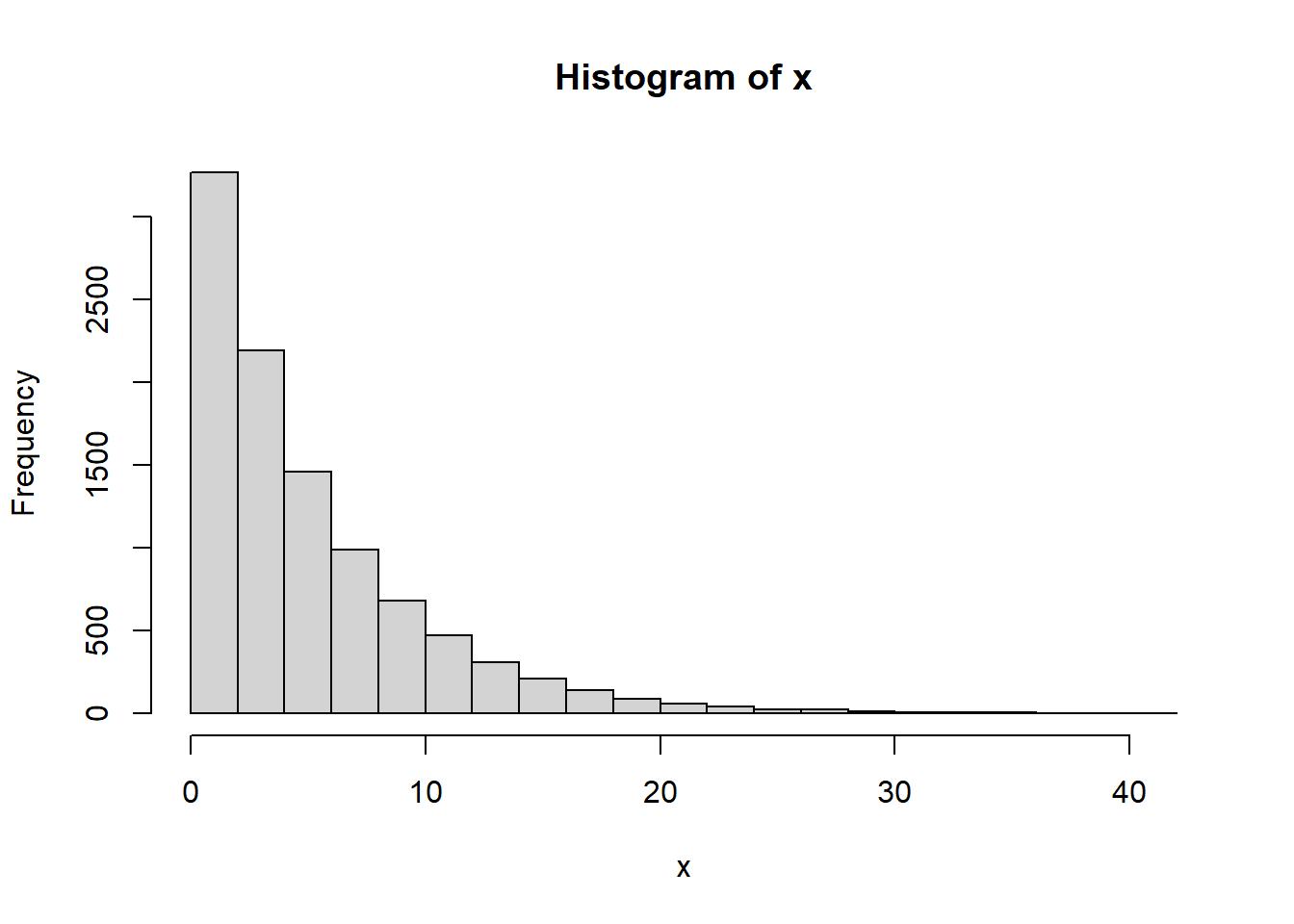
6.3.2 Random samples of size 10 with 500 draws
exp_means=c(1:500)
for (i in 1 : nsim){ exp_means[i] = mean(sample(x,10)) }
sample_mean<-mean(exp_means)
hist(exp_means,main="Histogram of 500 draws from exponential distribution",breaks=25,xlim = c(0,10))
abline(v = miu, col= 2, lwd = 2,lty=2)
abline(v = sample_mean, col= 3, lwd = 1)
legend('topright', c("Expected Mean", "Sample Mean"),
       lty= c(2,1),
        bty = "n", col = c(col = 2, col = 3))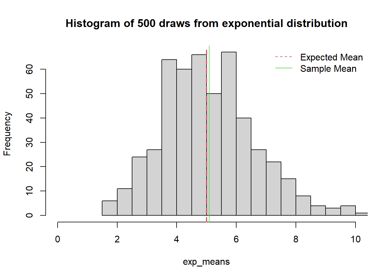
6.4 Sampling Distribution Properties
The expected value of the sample mean is the population mean. NOTE:E[a+b]=E[a]+E[b] \[E[\bar{x}]=E[\frac{1}{n}\sum{x_{i}}]=\frac{1}{n}\sum E[x_i]=\frac{1}{n}\sum \mu = \frac{1}{n}n\mu=\mu\]
The variance of the sample mean is dependent on the sample size and the population variance NOTE: if “a” is a constant and x has a variance of \(\sigma^2\), then \(VAR[a*x]=a^2 VAR[x]=a^2 \sigma^2\)
\[VAR[\bar{x}]=VAR[\frac{1}{n}\sum (x_i)]=\frac{1}{n^2}\sum VAR[x_i]=\frac{1}{n^2}*n*\sigma^2=\frac{\sigma^2}{n}\]
The standard error (SE) is the standard deviation of the sample mean. \[SE = \frac{\sigma}{\sqrt{n}}\] The standard error decreases if the sample size increases or the population standard deviation decreases.