Chapter 3 Math Review
- Summations
- Expected Value
- Central Limit Theorem
- Z score & T-statistics
- Derivatives
- Linear Algebra
3.1 Summations
In this class we will use a lot of math notation. One that will be used a great deal is the summation.
The summation symbol, denoted by the Greek letter sigma (Σ), has its origins in mathematics. It was introduced by the Swiss mathematician Leonhard Euler in the 18th century.
The symbol \(\sum\) is used to represent summation, which is a way of compactly expressing the addition of a sequence of numbers or terms. It is often used to represent the sum of a finite or infinite series. For example:
- The sum of the first n natural numbers can be written as: \(\sum_{i=1}^n i = 1 + 2 + 3 + ... + n\)
- The sum of the first n squares can be written as: \(\sum_{i=1}^n i^2 = 1 + 4 + 9 + ... + n^2\)
The symbol \(\sum\) is widely used in various branches of mathematics, physics, engineering, and other scientific fields to express summation in a concise and standardized manner. It has become an essential notation for representing and working with sums of sequences and series.
\[\sum^n_{i=1} x_i=x_1+x_2+x_3+...x_n\] This is a basic summation. It states there are n observations of x and we would like to sum all of those observations together.
What if x is a constant (think equal to one number)? \[\sum^n_{i=1} 2=2+2+2+...2=2n\]
3.1.1 Multiply a summation
Something common that happens is that we multiply x by a constant \(a\). \[a\sum^n_{i=1} x_i=ax_1+ax_2+ax_3+...ax_n\]
A place you will see this a lot is with the mean. In this case, the mean essentially sums up all of the values and multiplies it by 1/n. WHY? \[\frac{1}{n}\sum^n_{i=1} x_i=\frac{x_1}{n}+\frac{x_2}{n}+\frac{x_3}{n}+...\frac{x_n}{n}\]
We can think of 1/n as the constant.
If we had the three values 1, 2, 3 and we wanted to know the mean \[\frac{1}{3}+\frac{2}{3}+\frac{3}{3}=\frac{6}{3}=2\]
3.2 Weighted Average
We can also multiply our \(x_i\)’s with other items that vary by x.
Two examples:
- a weighted average is \[\sum^n_{i=1}Pr(x_i) x_i=Pr(x_1)x_1+Pr(x_2)x_2+Pr(x_3)x_3+...Pr(x_n)x_n\] where \(Pr(x_i)\) is the probability that \(x_i\) will be observed.
- The probabilities must sum to 1, \(\sum_{i=1}^n Pr(x_i)=1\)
- The previous mean we discuss is a special case of the weighted average where all of the \(Pr(x_i)=\frac{1}{n}\).
- a covariance has two variables using the same index. \[\frac{1}{n}\sum^n_{i=1}(y_i-\mu_y)(x_i-\mu_x)\]
3.2.1 Examples of Weighted Average
The mean \[\bar{x}=\frac{1}{n}\sum^{n}_{i=1} x_i\] is a special case of a weight average. In this case, the Pr(x)=1/n for all values of x.
Another example of a weighted average is your grade average. Remember that 60 percent of your grade is the in class assignments and 40 percent are your quiz scores.
\[\begin{align} Grade &= Pr(Quiz)*\text{AVG QUIZ} + Pr(HW)*\text{AVG HW} \\ &= 0.4*\text{AVG QUIZ} + 0.6*\text{AVG HW}\end{align}\]
3.3 The Expected Value operator, E[]
The expected value is typically the mean of a random variable.
Formally, the expected value of \(x\) depends on its distribution. If x has a discrete distribution, then we would use the weighted average on the previous slide.
If x is a continuous random variable with a probability density of function of \(f(x)\) is given by \[E[x]=\int^b_{a}x f(x)dx\]
In our class, you can primarily assume that x is normally distributed where the mean of x is given by \(\mu\) and the variance is given by \(\sigma^2\).
The standard normal is a special case where \(\mu=0\) and \(\sigma^2=1\).
3.3.1 Application of the E[x] Operator
Let’s look at the function for the mean. How do we know this function actually gives us the mean?
\[\bar{x}=\frac{1}{n}\sum x_i \rightarrow E[\bar{x}]=E[\frac{1}{n}\sum x_i ]\]
- Rule 1: The expected value of a constant is just the constant \(E[a]=a.\) Why? Well \(a\) is not random. It keeps it’s value.
- Rule 2: \(E[ax]=aE[x]\)
- Rule 3: if \(x\) and \(y\) are random, then \(E[x+y]=E[x]+E[y]\)
- Rule 4: \(E[x^2]\neq (E[x])^2\) \(\leftarrow\) important for variance.
Let’s prove that \(E[\bar{x}]=\mu\)
\(E[\bar{x}]=E[\frac{1}{n}\sum x_i ]=\frac{1}{n}E[\sum x_i ]\) by Rule 2. Here we recognize that \(1/n\) is just a constant.
\(E[\bar{x}]=\frac{1}{n}E[\sum x_i ]=\frac{1}{n}\sum E[x_i ]=\frac{1}{n}\sum \mu\) by Rule 3. Here we recognize that the expected value of sum is the same as the sum of the expected value.
You can think of \(\mu\) as a constant, \(E[\bar{x}]=\frac{1}{n}\sum \mu=\frac{1}{n}n \mu=\mu\)
__(Sidebar: population parameters like \(\mu\) and \(\sigma\) are constants, but sample statistics like \(\bar{x}\). We will talk more about this later.)
3.4 Variance operator, Var[x]
We can define the variance function, \(Var[x]=E[x^2]-(E[x])^2\). Recall Rule 4?
Sticking with the normality assumption \(Var[x]=\sigma^2\).
- Rule 5: If \(a\) is a constant, then \(Var[ax]=a^2Var[x]=a^2\sigma^2\).
- Rule 6: If x and y are random variables, then \(Var[x+y]=Var[x]+Var[y]+2COV[x,y]\)
- Rule 7: If x and y are random variables, then \(Var[x-y]=Var[x]+Var[y]-2COV[x,y]\) because \(Var[y]=Var[-y]\).
- Rule 8: If x and y are independent, \(COV[x,y]=0\)
3.4.1 Variance of the sample mean
Let’s try to find \(Var[\bar{x}]\)
\[Var[\bar{x}]=Var[\frac{1}{n}\sum x_i] = \frac{1}{n^2}\sum Var[x_i]= \frac{1}{n^2}\sum \sigma^2=\frac{\sigma^2}{n}\] Notice, the sample mean is unbiased in that \(E[\bar{x}]=\mu\) and as the sample size increases \(Var[\bar{x}]\rightarrow 0\).
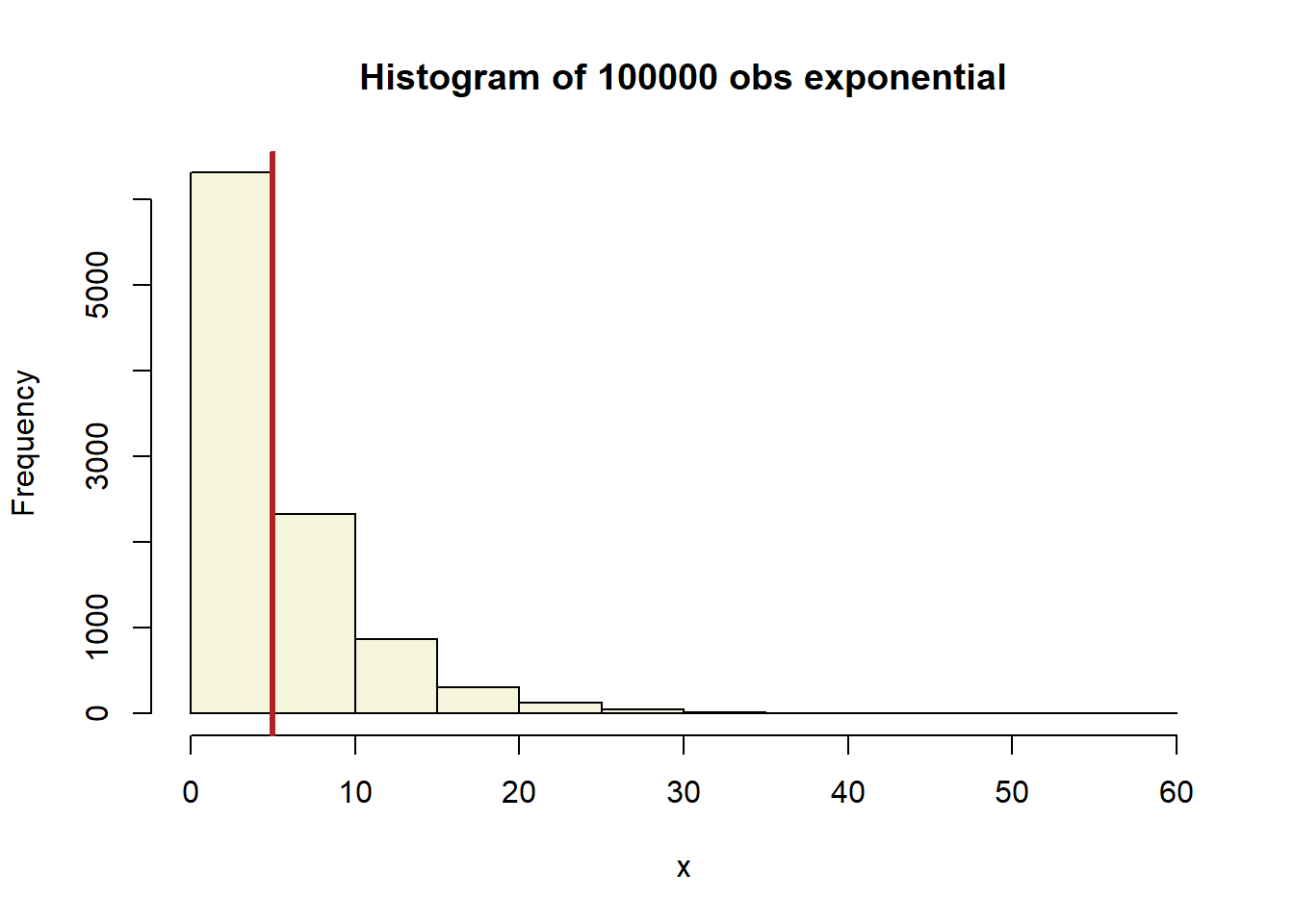
3.5 Central Limit Theorem
The Central Limit Theorem (CLT) says that the sample means from almost any distribution will be approximately normally distributed. Here we show an exponential distribution with a mean of 5. We used 10,000 draws from an exponential distribution to make this histogram.
3.5.1 CLT
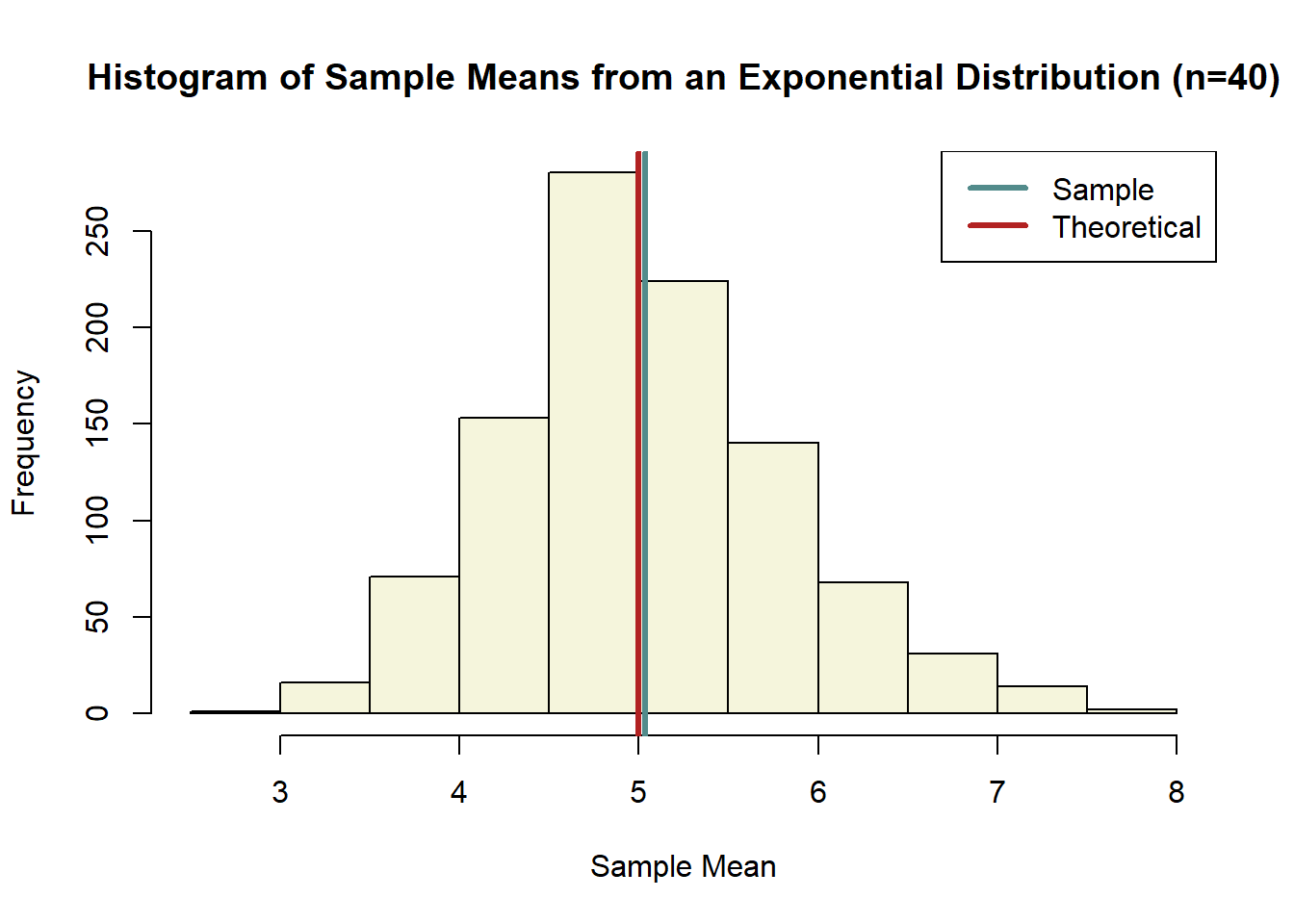
Here we take a random sample of size 40 from the exponential distribution, then we calculate the mean. We do this 1,000 times. Then we graphed a histogram of these 1,000 sample means. Notice, that the graph no longer looks like the original exponential. If any thing, it should look like a normal distribution. Also notice that the average sample mean across the 1000 observations is very close to the theoretical mean of the original exponential distribution.
3.5.2 CLT and Z-scores
- The CLT allows us to treat sample means like normally distributed random variables.
- A z-score is a way of transforming any normally distributed random variable into a standard normal random variable. \[Z=\frac{\text{observed x - mean of x}}{\text{std of x}}\]
- we subtract the mean so that the x is centered at zero. We divided by the standard deviation to force the new standard deviation to be 1.
- The z-score measures how far x is from zero using standard deviation as the size of the measurement (i.e. z = 2.3 means x is 2.3 standard deviations above zero)
Let’s say we are interested in the mean of x instead of x itself. Now our observed value is \(\bar{x}\), the population mean of x is \(\mu\) and we need the standard deviation of \(\bar{x}\). Remember, we calculated the variance of \(\bar{x}\) in section 3.4.1. Therefore, we an take the square root of variance of \(\bar{x}\) to get its standard deviation. Now plug that into the z-score formula and you get \[Z=\frac{\bar{x}-\mu}{\sigma / \sqrt{n} }\]
3.6 Z-scores and T-statistics
- We can use a Z-score only when we assume the random variable is normally distributed or the sample size is very large.
- In most cases, you will not use the z-score. Instead, you will use the t-statistics \[t=\frac{\bar{x}-\mu}{s / \sqrt{n} }\] where s is the sample standard deviation.
- You might be saying, “these don’t look that different.”
- The student T distribution has fatter tails. The fatter tails indicate more uncertainty. More uncertainty means wider confidence intervals.

“Ok, great, but what is the formula for the sample variance?” Glad you asked.
\[s^2 = \frac{1}{n-1}\sum (x_i -\bar{x})^2\]
You will notice that the sample variance divides by \(n-1\) instead of \(n\). This is the first time you run into the idea of “degrees of freedom”. Each time you use an estimate to find another estimate you lose a degree of freedom. It is like saying you use the same information twice. In this case, we estimate the population mean \(\mu\) using the sample mean \(\bar{x}\). Since \(\bar{x}\) is an estimate we lose a degree of freedom when calculating \(s^2\).
The sample standard deviation is just the square root of the variance, std x = \(\sqrt{s^2}=s\)
 - The term
 3.7 Basic Calculus
- This section is not meant to teach you calculus!!
- However, there are some basic concepts and formulas you will need.
- But first some algebra.
\[y=mx+b\] This is the standard formula for a line.
- \(x\) is the independent variable
- \(y\) is the dependent variable.
- \(m\) is the slope and tells us how y changes when x changes.
- \(b\) is the y-intercept \[y=\beta_0+\beta_1x\]
A simple linear regression takes essentially the same form
- \(\beta_0\) is the y intercept
- \(\beta_1\) is the slope
\[y=\beta_0+\beta_1x_1+\beta_2x_2\] Now we interpret the slopes differently
- \(\beta_1\) is the \(\Delta y\) when \(\Delta x_1\) holding \(x_2\) constant.
- \(\beta_2\) is the \(\Delta y\) when \(\Delta x_2\) holding \(x_1\) constant.
- notice we are assuming the other values are being held constant.
What about a non-linear function like \[y=\beta_0+\beta_1x_1+\beta_2x_1^2\] Now it is not so clear what the slope is of the line.
Non-Linear functions
\[y=\beta_0+\beta_1x_1+\beta_2x_1^2\] You have seen this function before in your algebra class. It looked like this instead. \[y=ax^2+bx+c\] and you learn the rule that if \(a>0\) this had a U shape to it else it \(\cap\).
You then learned a rule that the peak or trough of these U occurred when \[x=-\frac{b}{2a}\]
This rule comes from calculus.
Basic derivative
The derivative tells us the slope. It tells us how a change in x causes a change in y.
These are the formulas for your basic derivatives.
Rule 1: Let \(a\) be a constant and \(n\) be the value of an exponent. The simplest case is when \[y=a \rightarrow \frac{dy}{dx}=0\] The reason is that \(a\) is a constant and does not change with x; therefore y does not change.
Rule 2: A more common derivative is one with an exponent. \[y=ax^n \rightarrow \frac{dy}{dx} = anx^{n-1}\] A special case here is when \(n=1\), then we are given just a linear line and \(a\) is the slope.
You should be familiar with the marginal effect in linear regression when all the X’s enter linearly. But what about when the X’s enter in non-linearly? (Side bar: It is called linear regression because the \(\beta\)’s are linear. The X’s do not have to be.)
\[y=\beta_0+\beta_1x_1+\beta_2x_1^2\] We can find the marginal effect of x on y by taking a derivative. \[\frac{dy}{dx_1}=\beta_1+2\beta_2x_1\] The derivative of \(\beta_0\) is zero because it is a constant. The derivative of \(\beta_1x_1\) is \(\beta_1\) since it is the linear portion. The derivative of \(\beta_2x^2_1\) is \(2\beta_2x_1\) using our derivative formula.
The maximum or minimum of a parabola occurs when the slope is equals to zero (i.e. dy/dx = 0).\[\frac{dy}{dx_1}=\beta_1+2\beta_2x_1=0; \text{ solve for }x_1\]
\[x_1 = -\frac{\beta_1}{2\beta_2}\]
3.8 Linear Algebra
Matix multiplication \[\begin{bmatrix} a & b \\ c & d \end{bmatrix} \begin{bmatrix} e \\ f \end{bmatrix}=\begin{bmatrix} ae+bf \\ ce+df \end{bmatrix}\] Matrix Inversion - The matrix must be of full rank - The matrix must be square \[\begin{bmatrix} a & b \\ c & d \end{bmatrix}^{-1}=\frac{1}{ad-cb}\begin{bmatrix} d & -b \\ -c & a \end{bmatrix} \\ X^{-1}X=XX^{-1}=I \text{; I is the identity Matrix}\]
3.8.1 Multiple Regression in matrix form
Matrix notation is very useful to write regression equations. \[Y=\begin{bmatrix} y_1\\ y_2\\ ...\\ y_n \end{bmatrix}, X=\begin{bmatrix} 1 & x_{11} & x_{21} & \cdots & x_{k1} \\ 1 & x_{12} & x_{22} & \cdots & x_{k2}\\ \vdots & & & \\ 1 & x_{1n} & x_{2n} & \cdots & x_{kn} \end{bmatrix}, \beta =\begin{bmatrix} \beta_0\\ \beta_1\\ \vdots \\ \beta_k \end{bmatrix}, u=\begin{bmatrix} u_1\\ u_2\\ ...\\ u_n \end{bmatrix} \\ \\Y=X\beta+u\]
3.8.2 Multiple Regression in matrix form
We can actually solve for the \(\beta\)’s using matrix notation.
There are two key assumptions about the regression error.
- The mean of the error is zero.
- The X’s are independent of the error.
These two assumptions imply \[X'u = 0\]
So let’s use this fact to solve for \(\beta\). Pre-multiply everything in the regression equation by \(X'\).
\[\begin{align} X'Y &= X'X\beta+X'u \\ &= X'X\beta \\ (X'X)^{-1}X'Y &= (X'X)^{-1}X'X\beta \\ (X'X)^{-1}X'Y &= \beta \end{align}\]
This is what your computer is doing under the hood each time you run a regression.