Chapter 14 Linear Probability, Probit, Logit
- Previously, we learned how to use binary variables as regressors (independent variables)
- But in some cases we might be interested in learning how entity characteristics influence a binary dependent variable
- For example, we might be interested in studying whether there is racial discrimination in the provision of loans
- We are interested in comparing individuals who are identify with different races, but are otherwise identical
- It is not sufficient to compare average loan denial rates

We will consider two forms of regression to analyze such situations
- Linear Probability Models, using OLS to do multiple regression analysis with a binary dependent variable
- Nonlinear Regression Models, that might be a better fit of such binary models
The Math of Latent Dependent Variables
In economics, we believe people choose to do things that makes them better off. That is, they maximize utility.
Suppose you could go out to eat (option 1) or cook at home (option 2).
Each option gives you different utility. - \(u_1=X_1\beta+e_1\) is the utility you get from eating out - \(u_2=X_2\beta+e_2\) is the utility you get from cooking at home
Let \(y*\) represent a person’s net utility, \(y*=u_1-u_2\). We do not get to observe \(y*\).
Instead, we observe \(y=1\) if \(y*>0\) and \(y=0\) otherwise. - \(y=1\) implies you went out to each. - \(y=0\) implies you cooked at home.
We want to know the probability you go out to eat, \(Prob(y=1)\)
To calculate probability, we need to use a pdf and cdf - pdf = probability density function (gives the shape of the distribution) - cdf = cumulative density function
The blue line below is the pdf. We use the cdf to calculate probability that the z score is between \(z_1\) and \(z_2\) (the shaded region in yellow.)

\[y* = X \beta+ \epsilon\] Now assume \(F\) is the cumulative density function of \(\epsilon\) \[\begin{align*} Prob(y=1) &= Prob(y*>0) \\ &= Prob(X \beta + \epsilon>0) \\ &= Prob(\epsilon>-X \beta ) \\ &= 1-Prob(\epsilon<-X \beta ) \\ &= 1-F(-X \beta ) \end{align*}\]
If F is symmetric about 0, \[\begin{align*} Prob(y=1) &= 1-F(\epsilon<-X \beta ) \\ &= F(X \beta ) \end{align*}\]
14.1 The entire lecture in a nutshell
- If we do not assume a distribution for the error terms and use OLS to estimate Y
- \(Prob(y=1)=F(X \beta)=X \beta\) the equation is linear
- If we assume the errors are normally distributed, then we use Probit to estimate Y
- \(Prob(y=1)=F(X \beta)=\Phi(X \beta)\) the equation is nonlinear.
- If we assume the errors are logistic, then we use Logit to estimate Y
- \(Prob(y=1)=F(X \beta)=\Lambda(X \beta)\) the equation is nonlinear.
Simulation Example
# We will make some fake data
XA <- rnorm(1000)*5+20
XB <- rnorm(1000)*5+10
eA <- rnorm(1000)*5
eB <- rnorm(1000)*5
B <- 0.7
y_star <- (XA-XB)*B + eA - eB
y <- ifelse(y_star>0,1,0)
mean(y)
## [1] 0.793#Let's run a regression using both y_star and y
X = XA - XB # we can only identify relative effects
reg1 <-lm(y_star ~ X)
reg2 <- lm(y ~ X)
stargazer::stargazer(reg1,reg2, type = "html")| Dependent variable: | ||
| y_star | y | |
| (1) | (2) | |
| X | 0.710*** | 0.024*** |
| (0.031) | (0.002) | |
| Constant | -0.279 | 0.555*** |
| (0.382) | (0.020) | |
| Observations | 1,000 | 1,000 |
| R2 | 0.348 | 0.185 |
| Adjusted R2 | 0.347 | 0.184 |
| Residual Std. Error (df = 998) | 7.120 | 0.366 |
| F Statistic (df = 1; 998) | 532.688*** | 226.518*** |
| Note: | p<0.1; p<0.05; p<0.01 | |
Predict Y
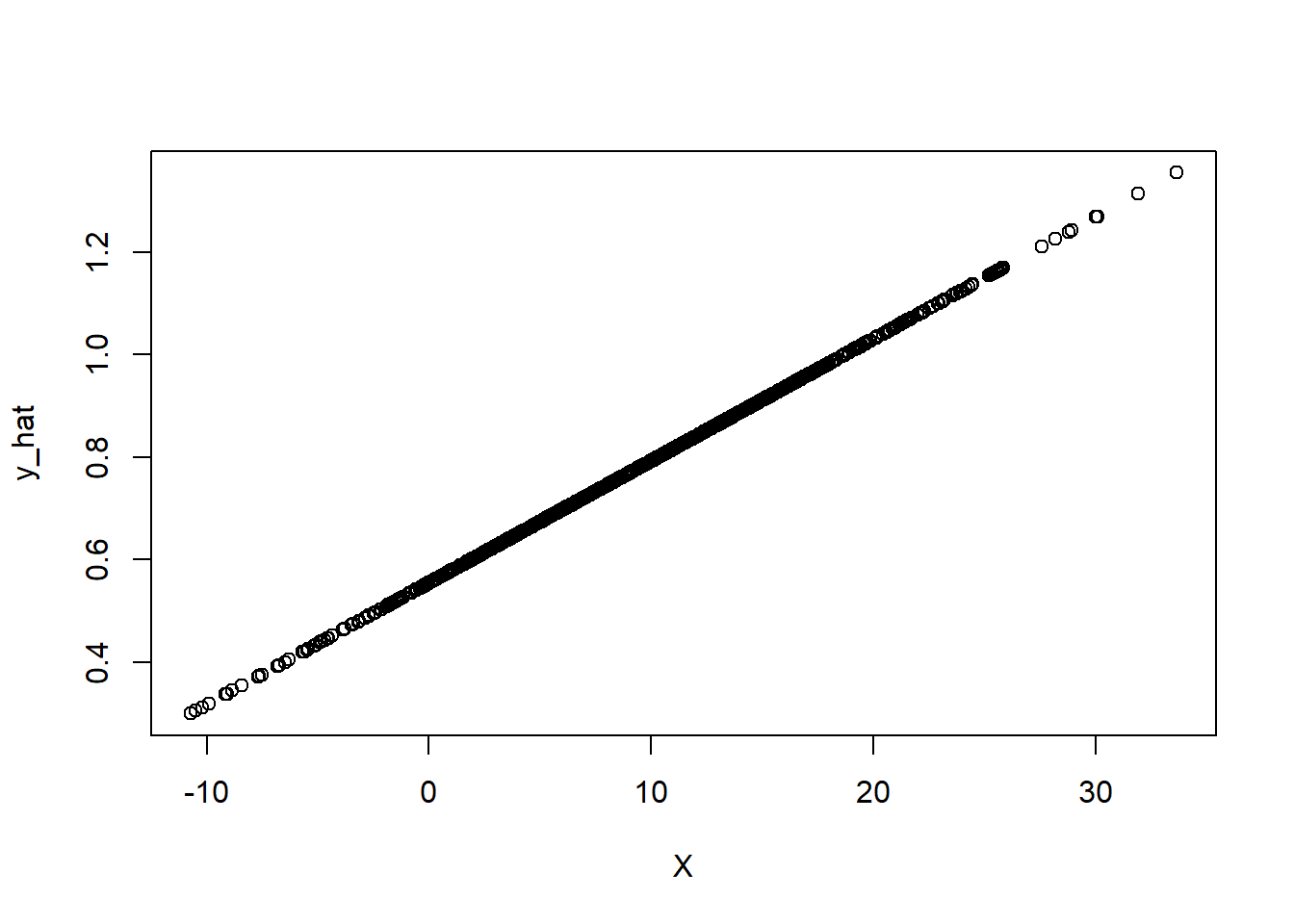
The predicted mean of y is 0.793, the max is 1.3552892, and the min is 0.2992141
14.2 Examples of Binary Dependent Variables
- The provision of a mortgage loan
- The decision to smoke/not smoke
- The decision to go to college or not
- If a country receives foreign aid or not
14.3 Redlining
Redlining is a discriminatory practice that involves denying or limiting access to certain services, such as housing, loans, or insurance, to individuals or communities based on their racial or ethnic background. The term “redlining” originated in the 1930s when the U.S. government and private lenders used red ink to mark neighborhoods on maps where they deemed loans too risky to approve, primarily based on the racial composition of the area.
Historical Background:
In the mid-20th century, government and private institutions engaged in redlining as part of housing and lending policies. The practice was prominent in the United States and targeted African American and other minority communities. Redlining resulted in systemic discrimination, racial segregation, and unequal access to housing and financial opportunities.
How Redlining Worked:
Redlining involved creating maps that categorized neighborhoods based on their perceived credit risk. Areas with high concentrations of African American, Hispanic, or other minority residents were often designated as “red” or “high-risk” zones. Banks and lenders would then use these maps to justify denying loans or offering unfavorable terms to residents and businesses in these neighborhoods.
Consequences of Redlining:
Housing Segregation: Redlining reinforced racial segregation by discouraging minorities from living in certain areas. It limited their housing options, leading to concentrations of poverty and limited access to quality education, healthcare, and other essential services.
Limited Access to Loans: Residents in redlined neighborhoods faced significant barriers in accessing mortgages and loans, making it challenging to purchase homes or start businesses.
Wealth Disparities: The lack of access to homeownership and loans contributed to the wealth gap between white communities and minority communities. Homeownership is a primary source of wealth accumulation, and redlining denied this opportunity to many minority families.
Long-Term Impact: The effects of redlining continue to be felt in many communities today. Redlined areas have historically been neglected in terms of investment and development, leading to persistent economic disparities.
Legislation and Mitigation:
Redlining was officially banned with the passage of the Fair Housing Act in 1968, which prohibited housing discrimination based on race, color, religion, sex, or national origin. However, its consequences persist to this day. Efforts to mitigate the impacts of redlining include community development initiatives, affordable housing programs, and advocacy for equitable lending practices.
Recognizing and addressing the historical legacy of redlining is crucial for promoting racial equity and social justice in housing and financial systems.
14.4 Racial Discrimination Mortgage Loans
- In this chapter we are interested in studying whether there is racial discrimination in the provision of mortgage loans.
- Data compiled by researchers at the Boston Fed under the Home Mortgage Disclosure Act (HMDA)
- The dependent variable of this example is a binary variable equal
- 1 if an individual is denied
- 0 otherwise
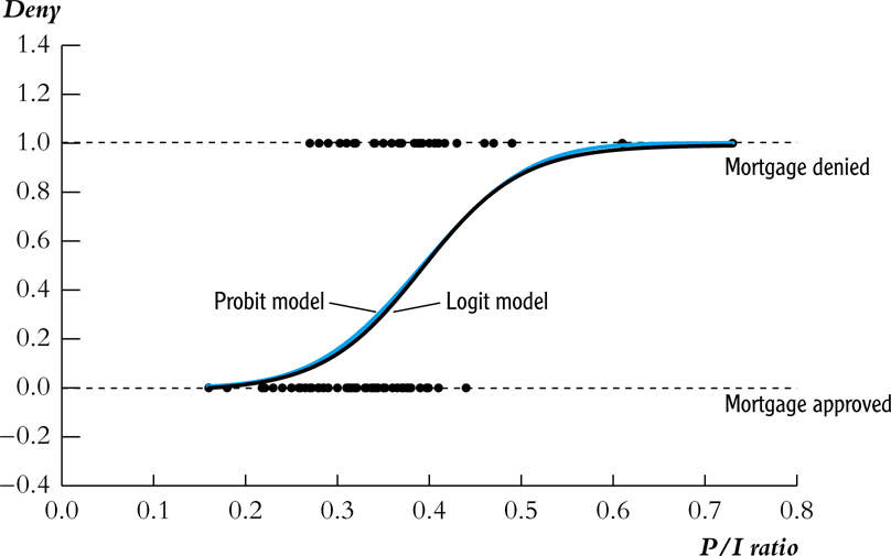
Effect of Payment-to-Income Ration
Using a subset of the data on mortgages \(n=127\)
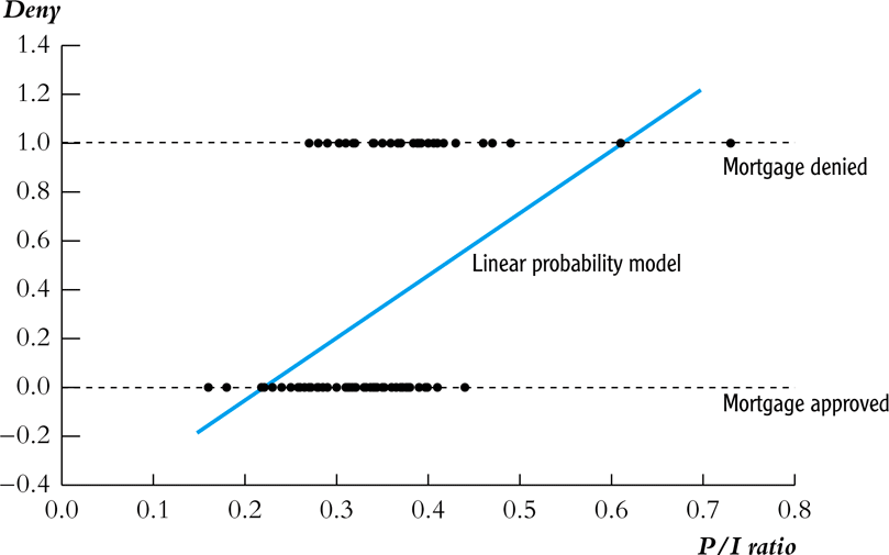
Interpreting the OLS Regression
Looking at the plot we see that when \(P/I~ratio = 0.3\), the predicted value \(\widehat{deny} = 0.2\).
What does it mean to predict a binary variable with a continuous value?
Using a probability linear model, we interpret this as predicting that someone with such a P/I ratio would be denied a loan with a probability of 20%.
The coefficients in the linear model tell us the marginal effect on the probability of getting denied a loan
14.4.1 The Linear Probability Model
The linear probability model is
\[Y_i = \beta_0 + \beta_1 X_{1i} + \dots + \beta_k X_{ki} + u_i\]
and therefore
\[Pr(Y = 1|X_1,\dots, X_k) = \beta_0 + \beta_1 X_{1} + \dots + \beta_k X_{k}\]
- \(\beta_1\) is the change in the probability that \(Y=1\) associated with a unit change in \(X_1\).
R Squared in a LPM
- A model with a continuous dependent variable one can imagine the possibility of getting \(R^2 = 1\), when all the data lines up on the regression line.
- This would be impossible if we had a binary dependent variable, unless the explanatory variables (X’s) are also all binary.
- Therefore, \(R^2\) from a LPM regression does not have a useful interpretation.
Application to the Boston HMDA Data
library(car)
library("AER")
data(HMDA)
fm1 <- lm(I(as.numeric(deny) - 1) ~ pirat, data = HMDA)

coeftest(fm1, vcov.=vcovHAC(fm1))
##
## t test of coefficients:
##
## Estimate Std. Error t value Pr(>|t|)
## (Intercept) -0.079910 0.032287 -2.4750 0.01339 *
## pirat 0.603535 0.102917 5.8643 5.138e-09 ***
## ---
## Signif. codes: 0 '***' 0.001 '**' 0.01 '*' 0.05 '.' 0.1 ' ' 1Application to the Boston HMDA Data
Note, once we control for an African American Family (afam), the likelihood of denial due to the PI ratio decreases. Further, we see a positive and significant effect on the afam variable
##
## t test of coefficients:
##
##              Estimate Std. Error t value  Pr(>|t|)
## (Intercept) -0.090514   0.029433 -3.0753  0.002127 **
## pirat        0.559195   0.091569  6.1068 1.184e-09 ***
## afamyes      0.177428   0.037471  4.7351 2.318e-06 ***
## ---
## Signif. codes:  0 '***' 0.001 '**' 0.01 '*' 0.05 '.' 0.1 ' ' 1
14.5 Introduction to Non-Linear Probability Model
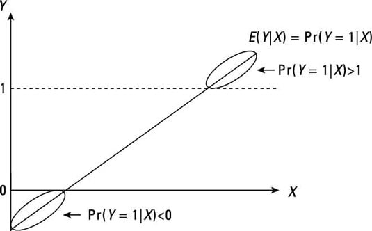
Since the fit in a linear probability model could be nonsensical, we consider two alternative nonlinear regression models
Since cumulative probability distribution functions (CDFs) produce functions from 0 to 1, we use them to model \(Pr(Y=1|X_1,\dots,X_k)\)
We use two types of nonlinear models
- Probit regressions, which uses the CDF of the standard normal
- Logit regression, uses a “logistic” CDF
14.6 Probit Regression
The Probit regression model with a single regressor is
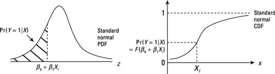
\[Pr(Y=1|X) = \Phi(\beta_0 + \beta_1 X)\]
where \(\Phi\) is the CDF of the standard normal distribution.
Probit uses a linear line to capture the Z-score, \(Z = \beta_0 + \beta_1 X\)
The CDF is nonlinear (remember what a normal distribution looks like), but the Z score is linear.
The normal CDF is non-linear
If \[y = \beta_0 + \beta_1 X + e,\]
then we know that if we increase X by one unit that the change in y will equal \(\beta_1\),
\(\delta y / \delta X = \beta_1\)
But the same is not true for either probit or logit.
Why is this important?
If you are moving from z = 2.0 to z = 3.0, then the change in probability is big, but from z = 3.0 to 4.0 is a much smaller change in probability even though the change in z is the same!!
# create a list of z values from -3 to 3 increasing by .1
z <- seq(-3,3, by = .1)
# We want to calculate the change in probability for a .1 change in z
z1 <- z[1:length(z)-1]
z2 <- z[2:length(z)]
y <- pnorm(z2)-pnorm(z1)
plot(z1,y)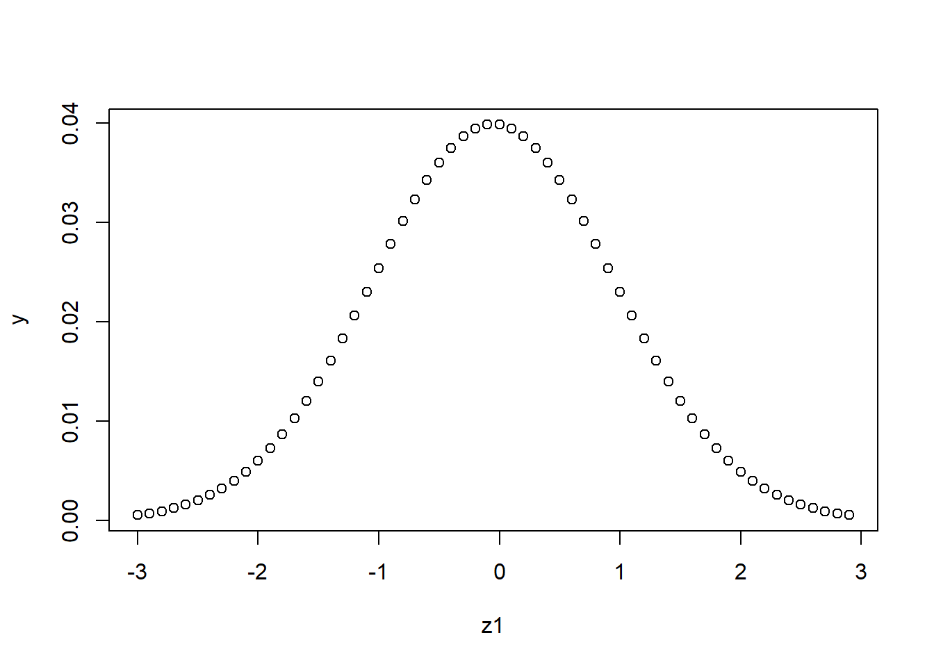
Graphic Representation of the problem.
Example
- Consider the mortgage example, regression loan denial on the P/I ratio
- Suppose that \(\beta_0 = -2\) and \(\beta_1 = 3\)
- What is the probability of being denied a loan is \(P/I~ratio = 0.4\)?
\[\begin{align*} \Phi(\beta_0 + \beta_1 P/I~ratio) &= \Phi(-2 + 3\times P/I~ratio)\\ &= \Phi(-0.8) \\ &= Pr(Z \leq -0.8) = 21.2\% \end{align*}\]where \(Z \sim N(0,1)\)
Interpreting the Coefficient
\[Pr(Y=1|X) = \Phi(\underbrace{\beta_0 + \beta_1 X}_{z})\]
- \(\beta_1\) is the change in the \(z\)-value associated with a unit change in \(X\).
- If \(\beta_1 > 0\), an increase in \(X\) would lead to an increase in the \(z\)-value and in turn the probability of \(Y=1\)
- If \(\beta_1 < 0\), an increase in \(X\) would lead to a decrease in the \(z\)-value and in turn the probability of \(Y=1\)
- While, the effect of \(X\) on the \(z\)-value is linear, its effect on \(Pr(Y=1)\) is nonlinear
Probit Model Graph

Multiple Regressors in Probit
\[Pr(Y=1|X_1, X_2) = \Phi(\beta_0 + \beta_1 X_1 + \beta_2 X_2)\]
- Once again the parameters \(\beta_1\) and \(\beta_2\) represent the linear effect of a unit change in \(X_1\) and \(X_2\), respectively, on the \(z\)-value.
- For example, suppose \(\beta_0 = -1.6\), \(\beta_1 = 2\), and \(\beta_2 = 0.5\). If \(X_1 = 0.4\) and \(X_2 = 1\), the probability that \(Y=1\) would be \(\Phi(-0.3) = 38\%\).
General Probit Model
\[\begin{equation*} Pr(Y=1|X_1, X_2,\dots, X_k) = \\ \\ \Phi(\underbrace{\beta_0 + \beta_1 X_1 + \beta_2 X_2 + \dots + \beta_k X_k}_z) \end{equation*}\]To calculate the effect of a change in a regressor (e.g. from \(X_1\) to \(X_1 + \Delta X_1\)) on the \(Pr(Y=1|X_1,\dots,X_k)\), subtract \[\Phi(\beta_0 + \beta_1 X_1 + \beta_2 X_2 + \dots + \beta_k X_k)\]from \[\Phi(\beta_0 + \beta_1 (X_1 + \Delta X_1) + \beta_2 X_2 + \dots + \beta_k X_k)\]
Application to Mortgage Data
##
## Call:
## glm(formula = deny ~ pirat, family = binomial(link = "probit"),
##     data = HMDA)
##
## Coefficients:
##             Estimate Std. Error z value Pr(>|z|)
## (Intercept)  -2.1941     0.1378 -15.927  < 2e-16 ***
## pirat         2.9679     0.3858   7.694 1.43e-14 ***
## ---
## Signif. codes:  0 '***' 0.001 '**' 0.01 '*' 0.05 '.' 0.1 ' ' 1
##
## (Dispersion parameter for binomial family taken to be 1)
##
##     Null deviance: 1744.2  on 2379  degrees of freedom
## Residual deviance: 1663.6  on 2378  degrees of freedom
## AIC: 1667.6
##
## Number of Fisher Scoring iterations: 6##
## Call:
## glm(formula = deny ~ pirat + afam, family = binomial(link = "probit"),
## data = HMDA)
##
## Coefficients:
## Estimate Std. Error z value Pr(>|z|)
## (Intercept) -2.25879 0.13669 -16.525 < 2e-16 ***
## pirat 2.74178 0.38047 7.206 5.75e-13 ***
## afamyes 0.70816 0.08335 8.496 < 2e-16 ***
## ---
## Signif. codes: 0 '***' 0.001 '**' 0.01 '*' 0.05 '.' 0.1 ' ' 1
##
## (Dispersion parameter for binomial family taken to be 1)
##
## Null deviance: 1744.2 on 2379 degrees of freedom
## Residual deviance: 1594.3 on 2377 degrees of freedom
## AIC: 1600.3
##
## Number of Fisher Scoring iterations: 514.7 Logit Regression
\[\begin{equation*} Pr(Y = 1|X_1, \dots, X_k) =\\ F(\beta_0 + \beta_1 X_1 + \dots + \beta_k X_k) =\\ \frac{1}{1+\exp(\beta_0 + \beta_1 X_1 + \dots + \beta_k X_k)} \end{equation*}\]
It is similar to the probit model, except that we use the CDF for a standard logistic distribution, instead of the CDF for a standard normal.
Probit vs Logit Regression Models
Application to Mortgage Data
##
## Call:
## glm(formula = deny ~ pirat + afam, family = binomial(link = "logit"),
##     data = HMDA)
##
## Coefficients:
##             Estimate Std. Error z value Pr(>|z|)
## (Intercept)  -4.1256     0.2684 -15.370  < 2e-16 ***
## pirat         5.3704     0.7283   7.374 1.66e-13 ***
## afamyes       1.2728     0.1462   8.706  < 2e-16 ***
## ---
## Signif. codes:  0 '***' 0.001 '**' 0.01 '*' 0.05 '.' 0.1 ' ' 1
##
## (Dispersion parameter for binomial family taken to be 1)
##
##     Null deviance: 1744.2  on 2379  degrees of freedom
## Residual deviance: 1591.4  on 2377  degrees of freedom
## AIC: 1597.4
##
## Number of Fisher Scoring iterations: 5
14.8 Marginal Effects
While it is straightforward to perform hypothesis testing on the \(\beta\)’s of a non-linear model, the interpretation of these coefficients are difficult.
Instead, we have a preference for marginal effects.
To find the marginal effects, we would need to take the derivative of the probability function and then find the expected value of the derivative.
To perform this task by hand is very difficult. Instead, we will use a package called mfx
Application to Mortgage Data
suppressMessages(library("mfx"))
fm6 <- probitmfx(deny ~ pirat, data = HMDA)
fm7 <- probitmfx(deny ~ pirat + afam, data = HMDA)
fm8 <- logitmfx(deny ~ pirat + afam,  data = HMDA)
texreg::htmlreg(list(fm3,fm6,fm2,fm7,fm8), custom.model.names = c("Probit","ME Probit","LPM","ME Probit", "ME Logit"),center = TRUE, caption = "", custom.note = "ME = Marginal Effect, LPM = linear probability model", omit.coef = c("aic","bic"))| Probit | ME Probit | LPM | ME Probit | ME Logit | |
|---|---|---|---|---|---|
| (Intercept) | -2.19*** | -0.09*** | |||
| (0.14) | (0.02) | ||||
| pirat | 2.97*** | 0.57*** | 0.56*** | 0.50*** | 0.49*** |
| (0.39) | (0.07) | (0.06) | (0.07) | (0.07) | |
| afamyes | 0.18*** | 0.17*** | 0.17*** | ||
| (0.02) | (0.02) | (0.02) | |||
| AIC | 1667.58 | 1667.58 | 1600.27 | 1597.39 | |
| BIC | 1679.13 | 1679.13 | 1617.60 | 1614.71 | |
| Log Likelihood | -831.79 | -831.79 | -797.14 | -795.70 | |
| Deviance | 1663.58 | 1663.58 | 1594.27 | 1591.39 | |
| Num. obs. | 2380 | 2380 | 2380 | 2380 | 2380 |
| R2 | 0.08 | ||||
| Adj. R2 | 0.08 | ||||
| ME = Marginal Effect, LPM = linear probability model | |||||
14.9 Advantages and Disadvantages
| Model Type | Advantages | Disadvantages |
|---|---|---|
| LPM | Can use fixed effects and easy to interpret | Can predict outside 0 and 1 |
| Probit | Prob. bounded between 0 and 1. | You can’t use fixed effects and suffers from incidental parameter problem. Coefficients are also hard to interpret. |
| Logit | Prob. bounded between 0 and 1. Can use one-way fixed effects (conditional logit) | Suffers Incidental parameter problem. Coefficients are hard to interpret. |
14.11 Limited Dependent Variables
Any time you have a non-continuous dependent variable, y, you will face some estimation challenges.
Some Examples
- The dependent variable is a dummy variable
- This represents a simply yes/no choice
- Did you buy the good?
- Did you accept the job?
- Did you get married?
- Did you get divorced?
- Did you move?
- Did you vote?
- Did you get a flu shot?
We can estimate the likelihood of making one of these choices using - LPM: Linear Probability Model - Probit: Non-linear Model which assumes a normally distributed error - Logit: Non-linear Model which assumes a logistic distributed error.
14.11.1 More than one choice
Sometimes, we can represent multiple choices
Examples,
- Full-Time Employment, Part-time Employment, Unemployed, out of the labor force
- College Major
- Occupational Choice
- Type of cereal
We use Multinomial Logit or Probit (Future Class)
14.11.2 Discrete Counts
Sometimes, we have discrete amounts of an item
- Number of kids
- Number of shoes
- Number of suicides
- Number of businesses
These are examples of count variables Models used are Poisson and Negative Binomial (Future class)
14.11.3 Limited Dependent Variables and Choice Theory
The one key insight of limited dependent variables is how well it fits in with Choice Theory.
Suppose you have two products, A and B. Which one will you buy first?
Choice Theory says you buy the good that gives you the most utility.
If \(U_A > U_B\) you buy A else you buy B.
We can define these utility functions as linear where \(X_A\) contains the observed characteristics of good A and \(X_B\) the observed characteristics of good B.
\(U_A = X_A\beta+e_A\) is your utility for good A
\(U_B = X_B\beta+e_B\) is your utility for good B
The error terms \(e_A\) and \(e_B\) represent the unobserved characteristics for the products that the statistician cannot observed, but the consumer can.
The product error terms are random variables. Therefore, we cannot know definitely if \(U_A > U_B\), but we can say what is the probability the consumer will choose product A over product B.
We do this by first defining a latent variable, \(y^*\). This latent variable is unobserved, but the choice Y is observed.
If \(y^* > 0\), then Y = 1 else Y = 0.
We know that the consumer choose product A if \(U_A > U_B\).
This is the same as saying \(y^*=U_A - U_B > 0\)
So \(y^* = (X_A-X_B)\beta+e_A-e_B\)
Similar to dummy variables, we cannot estimate the absolute effect when comparing two products. We can only estimate the relative effect.
Just as in the dummy variable case, we will need to set the utility of one of the goods to zero.
14.11.4 Probabilty
What is the probability the consumer buys good A?
First, let Y = 1 if the consumer buys good A. Also, let \(X = X_A-X_B\).
\[Pr(Y=1)=Pr(y^*>0)=Pr(X\beta+e_A-e_B>0)\]
Remember, X is just data that we observed.
\(\beta\) is the parameter we are interested in.
But the difference in the error terms is a random variable.
14.11.5 LPM
If we treat the difference of the error terms to have a mean zero and a constant variance, then we can run OLS on the equation. \[Y = X\beta+e_A-e_B\]
The coefficients would tells us by how many percentage points would the probability increase or decrease.
Sidebar: There is a difference between percent change and percentage point change. For example, if you move from 1% to 2% this is one percentage point change, but a 100% percent change.
14.11.6 Benefits and Problems of LPM
The benefit of this model is that you can apply all of the least squares techniques you have learned. - OLS - Fixed Effects - IV
The disadvantage is that it can predict probabilities greater than 1 and less than zero.
14.11.7 Benefits and Problems of LPM
The error of LPM
You will also have heteroscedastic errors in all cases.
You MUST always use robust standard errors in LPM models.
14.11.8 Probabilty
Instead, if we assume the difference in the error terms is distributed \(f(x)\) where \(F(x)\) is the cumulative probability function, then
\[Pr(Y=1)=Pr(y^*>0)=Pr(X\beta+e_A-e_B>0)\] \[Pr(Y=1)=Pr(X\beta+e_A-e_B>0)=Pr(e_A-e_B > -X\beta)\] \[Pr(Y=1)=Pr(e_A-e_B > -X\beta)= 1 - Pr(-X\beta > e_A-e_B)\]
\[Pr(Y=1)= 1 - Pr(-X\beta > e_A-e_B)= 1 - F(-X\beta)\] If we further assume that \(F(x)\) is symmetric (think of the normal distribution), then \[1 - F(-X\beta)=F(X\beta)\] So the probability that a consumer chooses to buy product A is \(Pr(Y=1|X)=F(X\beta)\) and the probability they choose product B is \(Pr(Y=0|X)=1-F(X\beta)\)
How do we estimate this function?
We will use a new estimation method to called Maximum Likelihood to estimate the \(\beta's\).
Suppose that we have three consumers.
- Consumer 1 buys product A.
- Consumer 2 buys product B.
- Consumer 3 buys product A.
What is the probability of observing this sequence?
If the consumers are making choices independently, then it is just the multiplication of their individual probabilities
\[L = Pr(Y=1|X)*Pr(Y=0|X)*Pr(Y=1|X)\] We write this same equation using the CDF function instead. \[L = F(X\beta)*[1-F(X\beta)]*F(X\beta))\]
We estimate \(\beta\) by searching for the value of \(\beta\) that maximizes \(L\).
If we had \(n\) consumers, then \(L\) would generalize to \[L=\Pi_i^n F(X_i\beta)^{Y_i}*[1-F(X_i\beta)]^{1-Y_i}\]
When the error terms, \(e_A\) and \(e_B\), are distributed normal, then the differences between the error terms, \(e_A-e_B\) is also normally distributed. We can then use the normal cumulative density function for \(F(x)\) \[F(X\beta)=\Phi(\frac{X\beta}{\sigma})=\Phi(X\beta)\]
Probit When the error terms are distributed normal the cumulative density function for \(F(x)\) \[F(X\beta)=\Phi(\frac{X\beta}{\sigma})=\Phi(X\beta)\]
We cannot separately identify the standard deviation \(\sigma\) from \(\beta\) so we assume \(\sigma\) is equal to one.
For example, the computer cannot tell the difference between \(\beta=2\) and \(\sigma=1\) versus \(\beta=4\) and \(\sigma=2\).
Logit
When the error terms are distributed Type I extreme value, then the differences in the error terms is logistic.
The logistic distribution is probably new to you. It has a computation advantage over the assumption of normally distributed errors. The CDF for the normal distribution has NO CLOSED FORM SOLUTION.
The logistic cdf has a very simple closed form solution. \[F(X\beta)=\frac{exp(X\beta)}{1+exp(X\beta)}\]
Similar to Probit, we have to assume the standard deviation is equal to one to identify \(\beta\).
Advantages of Probit and Logits vs LPM
Both Probit and Logit are bounded between 0 and 1.
LPM can give negative probabilities and probabilities greater than 1.
Both Probit and Logit do not have issues with heteroscedacity because of the functional form.
LPM can only have heteroscedastic errors.
You can use fixed effects with Logit (and sort of with Probit), but the estimation is more complex than in the LPM case.
Disadvantage of Probit/Logit A disadvantage of Probit/Logit is that parameters are difficult to interpret. We need to use marginal effects (derivative) to make any sense in these non-linear models.
We cannot easily incorporate fixed effects
Rule of Thumb: if the average probability of an event is far from the tails, then using LPM is just as good as using Logit or Probit and the interpretation is easier.