Chapter 13 Regression Discontinuity Design
13.1 Quick Review of diff-in-diff
This document replicates the Table 4.1 and Figures 4.2 4.4 4.5 found in Mastering Metrics (based on data from Carpenter and Dobkin 2009)
Will adding controls affect diff-in-diff estimates if treatment assignment was random?
- Answer = Not unless you’ve added ‘bad controls’, which are controls also affected by treatment.
When you’ve done this, you’re no longer estimating the causal effect of treatment
- Control (that are exogenous) will just improve precision, but shouldn’t affect estimates
What are some standard falsification tests you might want to run with diff-in-diff?
Answer
- Compare ex-ante characteristics of treated & untreated
- Check timing of treatment effect
- Run regression using dep. variables that shouldn’t be affected by treatment (if it is what we think it is)
- Check whether reversal of treatment has opposite effect
- Triple-difference estimation
If you find ex-ante differences in treated and treated, is internal validity gone?
- Answer = Not necessarily but it could suggest non-random assignment of treatment that is problematic. E.g. observations with characteristic ‘z’ are more likely to be treated and observations with this characteristic are also likely to be trending differently for other reasons
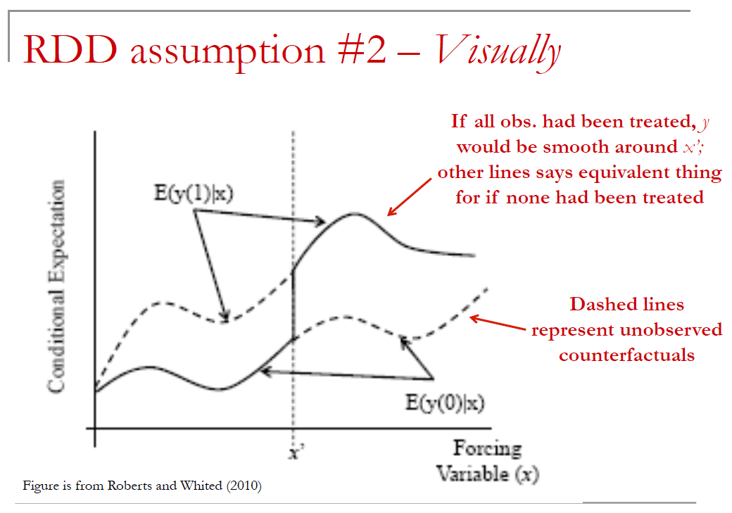
Does the absence of a pre-trend in diff-in-diff ensure that differential trends assumption holds and causal inferences can be made?
Answer = Sadly, no. We can never prove causality with 100% confidence. It could be that trend was going to change after treatment for reasons unrelated to treatment
How are triple differences helpful and reducing concerns about violation of parallel trends assumption?
Answer = Before, an “identification policeman” would just need a story about why treated might be trending differently after event for other reasons. Now, he/she would need story about why that different trend would be particularly true for subset of firms that are more sensitive to treatment
13.2 Basic idea of RDD
The basic idea of regression discontinuity RDD is the following:
- Observations (e.g. firm, individual, etc.) are “treated” based on a known cutoff rule.
- The cutoff is what creates the discontinuity.
Researcher is interested in how this treatment affects outcome variable of interest, \(y\).
Examples of RDD settings
- If you think about it, these type of cutoff rules are commonplace in finance
- A borrower FICO score > 620 makes securitization of the loan more likely
- Keys, et al (QJE 2010)
- A borrower FICO score > 620 makes securitization of the loan more likely
- Accounting variable x exceeding some threshold causes loan covenant violation
- Roberts and Sufi (JF 2009)
RDD is like difference-in-difference
- Has similar flavor to diff-in-diff natural experiment setting in that you can illustrate identification with a figure
- Plot outcome y against independent variable that determines treatment assignment, x.
- Should observe sharp, discontinuous change in y at the cutoff value of x.
But, RDD is different
- RDD has some key differences.
- Assignment to treatment is NOT random;
- Assignment is based on value of x
- When treatment only depends on x (what I’ll later call “sharp RDD”, there is no overlap in treatment & controls; i.e. we never observe the same x for a treatment and a control)
Randomized Experiment
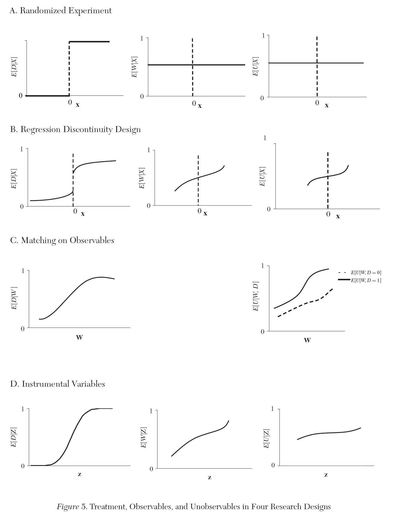
RDD randomization assumption
- Assignment to treatment and control isn’t random, but whether individual observation is treated is assumed to be random.
- i.e. researcher assumes that observations (e.g. firm, person, etc.) can’t perfectly manipulate their x value
- Therefore, whether an observation’s x falls immediately above or below key cutoff x is random
13.3 Two types of RDD
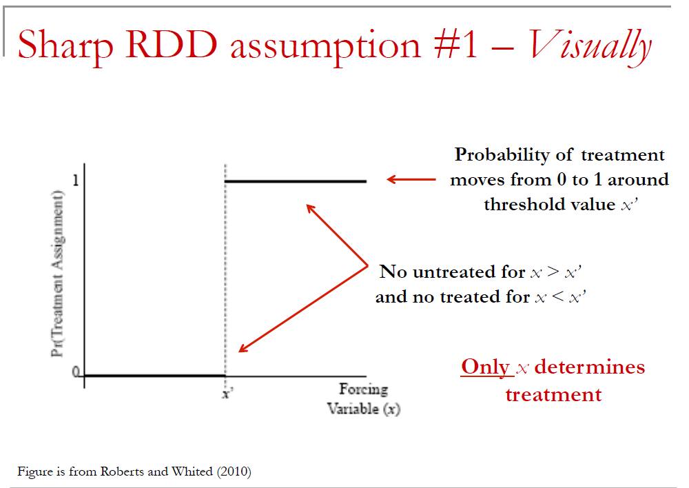
Sharp RDD
- Assignment to treatment only depends on x; i.e. if \(x >= x'\) you are treated with probability 1
Fuzzy RDD
- Having \(x >= x'\) only increases probability of treatment; i.e. other factors (besides x) will influence whether you are actually treated or not

13.3.3 Sharp versus Fuzzy RDD
This subtle distinction affects exactly how you estimate the causal effect of treatment
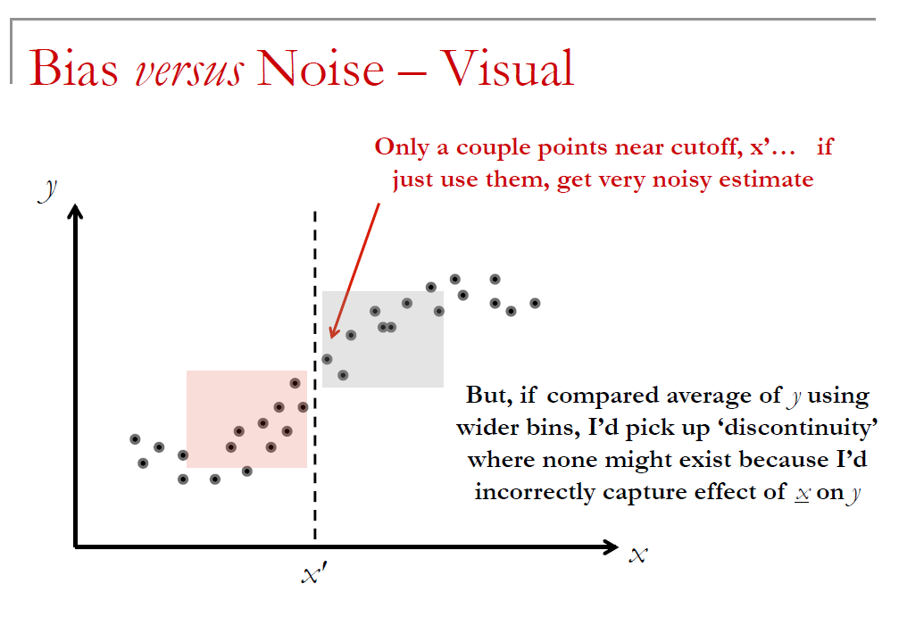
With Sharp RDD, we will basically compare average \(y\) immediately above and below \(x'\)
With fuzzy RDD, the average change in y around the threshold understate causal effect [why?]
- Answer = Comparision assumes all observations were treated, but this isn’t true; if all observations had been treated, observed change in y would be even larger; we will need to rescale based on change in probability
Parrallel Trends Assumption
13.3.4 Bias vs Noise
RDD Animated
 ## Simulated Data
Below is an example with no discontinuity. We force it this way by making X a uniformly distributed random variable from -1 to 1.
## Loading required package: Formula# you only need the running variable and the cutoff point
# Example by the package's authors
#No discontinuity
x<-runif(1000,-1,1)
DCdensity(x,0)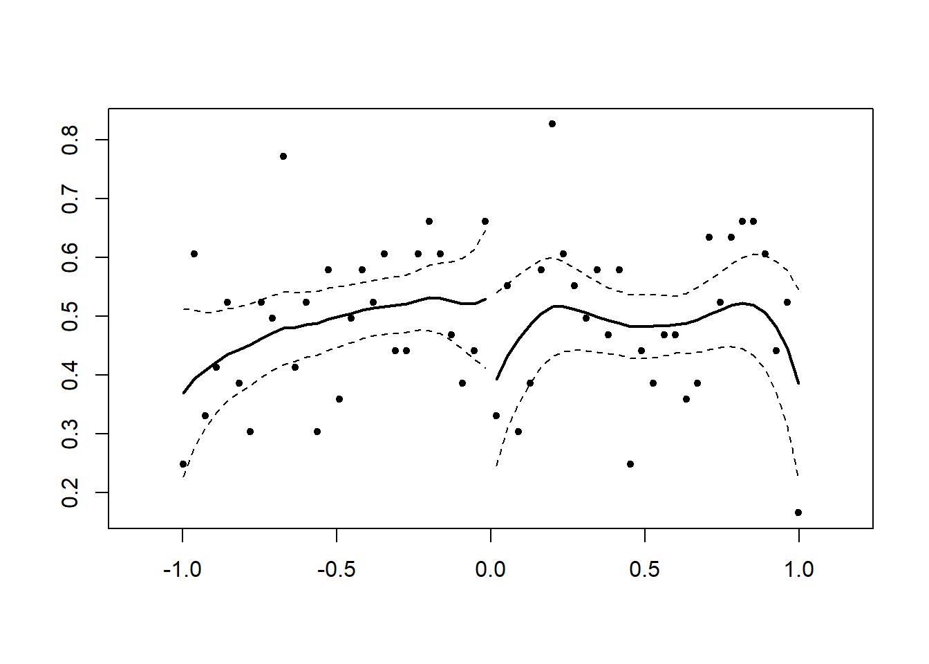
## [1] 0.1286819Now we can create a series with a discontinuity. We multiply the values of x by 2 if they are beyond the cutoff.
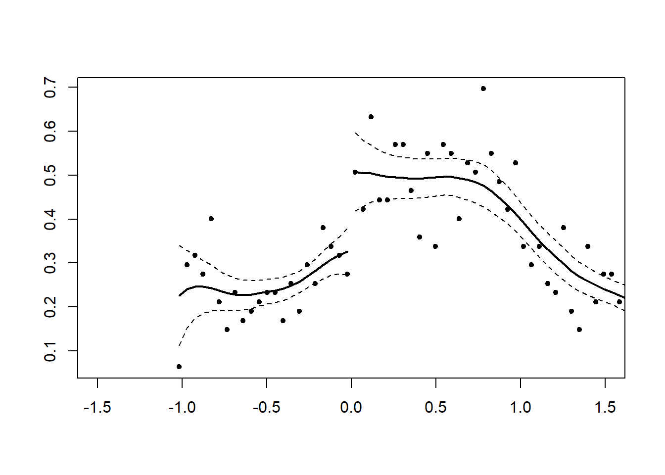
## [1] 0.0462568113.4 RDD in R
library(AER)
library(foreign)
library(rdd)
library(stargazer)
AEJfigs=read.dta("AEJfigs.dta")
# All = all deaths
AEJfigs$age = AEJfigs$agecell - 21
AEJfigs$over21 = ifelse(AEJfigs$agecell >= 21,1,0)
reg.1=RDestimate(all~agecell,data=AEJfigs,cutpoint = 21)
plot(reg.1)
title(main="All Causes of Death", xlab="AGE",
      ylab="Mortality rate from all causes (per 100,000)")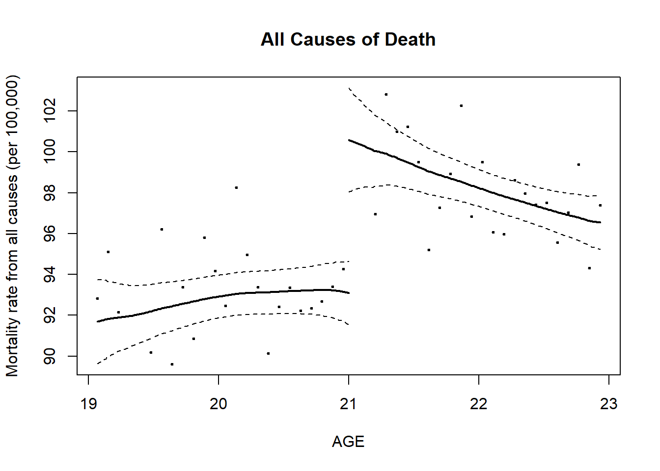
##
## Call:
## RDestimate(formula = all ~ agecell, data = AEJfigs, cutpoint = 21)
##
## Type:
## sharp
##
## Estimates:
##            Bandwidth  Observations  Estimate  Std. Error  z value  Pr(>|z|)
## LATE       1.6561     40            9.001     1.480       6.080    1.199e-09
## Half-BW    0.8281     20            9.579     1.914       5.004    5.609e-07
## Double-BW  3.3123     48            7.953     1.278       6.223    4.882e-10
##
## LATE       ***
## Half-BW    ***
## Double-BW  ***
## ---
## Signif. codes:  0 '***' 0.001 '**' 0.01 '*' 0.05 '.' 0.1 ' ' 1
##
## F-statistics:
##            F      Num. DoF  Denom. DoF  p
## LATE       33.08  3         36          3.799e-10
## Half-BW    29.05  3         16          2.078e-06
## Double-BW  32.54  3         44          6.129e-11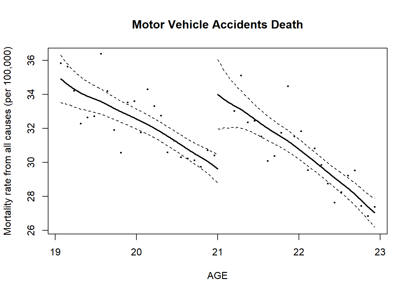
##
## Call:
## RDestimate(formula = mva ~ agecell, data = AEJfigs, cutpoint = 21)
##
## Type:
## sharp
##
## Estimates:
##            Bandwidth  Observations  Estimate  Std. Error  z value  Pr(>|z|)
## LATE       1.2109     30            4.977     1.0590      4.700    2.607e-06
## Half-BW    0.6054     14            4.956     1.3767      3.600    3.182e-04
## Double-BW  2.4218     48            4.566     0.7086      6.444    1.162e-10
##
## LATE       ***
## Half-BW    ***
## Double-BW  ***
## ---
## Signif. codes:  0 '***' 0.001 '**' 0.01 '*' 0.05 '.' 0.1 ' ' 1
##
## F-statistics:
##            F      Num. DoF  Denom. DoF  p
## LATE       13.32  3         26          3.692e-05
## Half-BW    12.76  3         10          1.879e-03
## Double-BW  26.99  3         44          9.322e-10
##
## Call:
## RDestimate(formula = internal ~ agecell, data = AEJfigs, cutpoint = 21)
##
## Type:
## sharp
##
## Estimates:
##            Bandwidth  Observations  Estimate  Std. Error  z value  Pr(>|z|)
## LATE       0.8809     22            1.4128    0.8206      1.722    0.08513   .
## Half-BW    0.4405     10            1.8691    1.0203      1.832    0.06698   .
## Double-BW  1.7618     42            0.7652    0.6179      1.239    0.21553
## ---
## Signif. codes:  0 '***' 0.001 '**' 0.01 '*' 0.05 '.' 0.1 ' ' 1
##
## F-statistics:
##            F       Num. DoF  Denom. DoF  p
## LATE        6.830  3         18          5.734e-03
## Half-BW     1.765  3          6          5.068e-01
## Double-BW  22.695  3         38          2.750e-08
13.5 Business Application of RDD Model
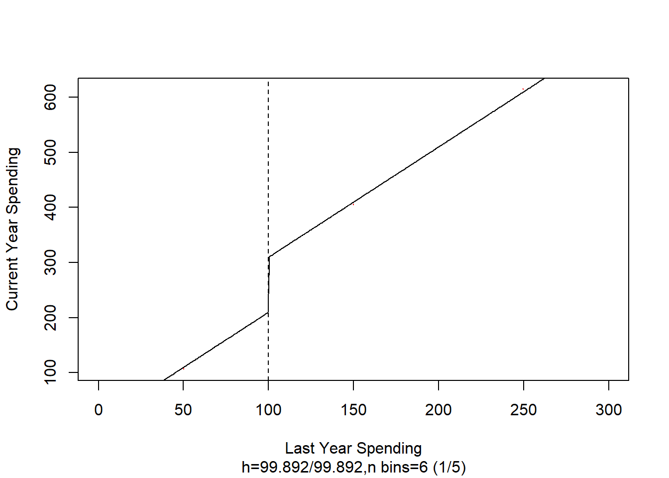
Let’s say a company is considering implementing a customer loyalty program and wants to assess its impact on customer spending. They decide to use regression discontinuity to analyze the data.
In this scenario, the company could set a specific spending threshold (e.g., $100) to qualify for the loyalty program. Customers who spend just below this threshold wouldn’t qualify, while those who spend just above would.
By comparing the spending behavior of customers who barely qualify for the loyalty program (just above the threshold) with those who barely miss qualifying (just below the threshold), the company can use regression discontinuity to estimate the causal effect of the loyalty program on customer spending. This helps them determine whether the loyalty program has a significant impact on increasing customer spending and overall revenue.
## Loading required package: np## Nonparametric Kernel Methods for Mixed Datatypes (version 0.60-17)
## [vignette("np_faq",package="np") provides answers to frequently asked questions]
## [vignette("np",package="np") an overview]
## [vignette("entropy_np",package="np") an overview of entropy-based methods]##
## Attaching package: 'np'## The following object is masked from 'package:fixest':
##
## se##
## Please consider citing R and rddtools,
## citation()
## citation("rddtools")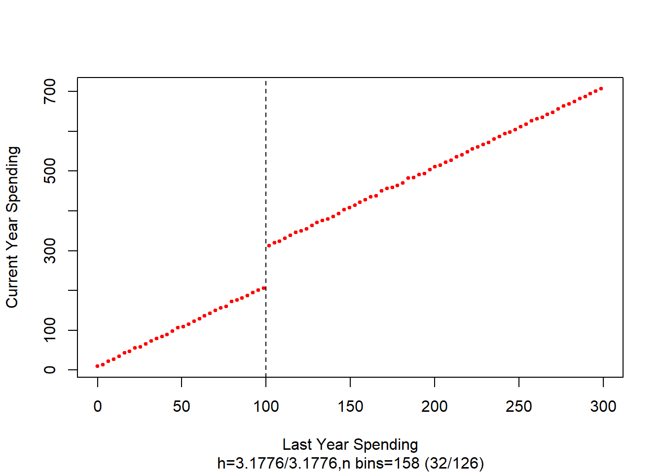
Let’s evaluate the effect of this loyalty program on consumer expenditures. We know the cutoff is at $100. We will use a regression based model to see if a combination of last year’s expenditures and the loyalty program increased current year expenditures. To increase your exposure to rdd packages, we will use rddtools
library(rddtools)
data <- rdd_data(future_year, current_year, cutpoint = 100)
# estimate the sharp RDD model
rdd_mod <- rdd_reg_lm(rdd_object = data, slope =  "same")
summary(rdd_mod)
##
## Call:
## lm(formula = y ~ ., data = dat_step1, weights = weights)
##
## Residuals:
## Min 1Q Median 3Q Max
## -12.5414 -2.5371 -0.0104 2.5993 11.9786
##
## Coefficients:
## Estimate Std. Error t value Pr(>|t|)
## (Intercept) 2.101e+02 2.477e-01 848.2 <2e-16 ***
## D 9.977e+01 4.597e-01 217.0 <2e-16 ***
## x 2.002e+00 2.447e-03 817.9 <2e-16 ***
## ---
## Signif. codes: 0 '***' 0.001 '**' 0.01 '*' 0.05 '.' 0.1 ' ' 1
##
## Residual standard error: 3.943 on 997 degrees of freedom
## Multiple R-squared: 0.9997, Adjusted R-squared: 0.9997
## F-statistic: 1.543e+06 on 2 and 997 DF, p-value: < 2.2e-16# plot the RDD model along with binned observations
plot(
rdd_mod,
cex = 0.1,
col = "red",
xlab = "Last Year Spending",
ylab = "Current Year Spending"
)


13.7 References
C. Carpenter and C. Dobkin, “The Effect of Alcohol Consumption on Mortality: Regression Discontinuity Evidence from the MLDA”, American Economic Journal: Applied Economics 1 (2009), 164-182.
A. Abdulkadiroglu, et al., “The Elite Illusion: Achievement Effects at Boston and New York Exam Schools”, Econometrica, 2014.