Chapter 9 Linear Regression
9.1 Introduction to Simple Linear Regression
- We are interested in the causal relationship between two random variables \(X\) and \(Y\)
- We assume that \(X\) (the regressor or the independent variable) causes changes in \(Y\) (the dependent variable)
- We assume that the relationship between them is linear
- We are interested in estimating the slope of this linear relationship
Example: The Effect of Class Size on Student Performance
- Suppose the superintendent of an elementary school district wants to know the effect of class size on student performance
- She decides that test scores are a good measure of performance

What she wants to know is what is the value of \[\beta_{ClassSize} = \frac{\text{change in }TestScore}{\text{change in }ClassSize} = \frac{\Delta TestScore}{\Delta ClassSize}\] If we knew \(\beta_{ClassSize}\) we could answer the question of how student test scores would change in response to a specific change in the class sizes \[\Delta TestScore = \beta_{ClassSize} \times \Delta ClassSize\] If \(\beta_{ClassSize} = -0.6\) then a reduction in class size by two students would yield a change of test scores of \((-0.6)\times(-2) = 1.2\).
Linear Equation of Relationship
\(\beta_{ClassSize}\) would be the slope of the straight line describing the linear relationship between \(TestScore\) and \(ClassSize\)
\[TestScore = \beta_0 + \beta_{ClassSize} \times ClassSize\]
If we knew the parameters \(\beta_0\) and \(\beta_{ClassSize}\), not only would we be able to predict the change in student performance, we would be able to predict the average test score for any class size
We can’t predict exact test scores since there are many other factors that influence them that are not included
- teacher quality
- better textbooks
- different student populations
- etc.
Our linear equation in this case is
\[TestScore = \underbrace{\beta_0 + \beta_{ClassSize} \times ClassSize}_{\text{Average }TestScore} + \text{ other factors}\] General Form
More generally, if we have \(n\) observations for \(X_i\) and \(Y_i\) pairs
\[Y_i = \beta_0 + \beta_1 X_i + u_i\]
- \(\beta_0\) (intercept) and \(\beta_1\) (slope) are the model parameters
- \(\beta_0 + \beta_1 X_i\) is the population regression line (function)
- \(u_i\) is the error term.
- It contains all the other factors beyond \(X\) that influence \(Y\). We refer to this relationship as: \(Y_i\) regressed on \(X_i\)
- In our case, \(Y_i\) is the average test score and \(X_i\) is the average class size, for district \(i\).
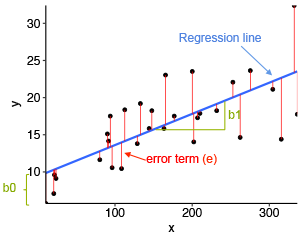
Regression Model Plot
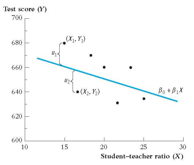
Notice from the plot that the errors, \(u_i\), are the distance between the line and the actual observation. We want to draw a line through the scatter plot that minimizes the errors across all observations.
Parameter Estimation
Our model
\[Y_i = \beta_0 + \beta_1 X_i + u_i\]
We don’t know the parameters \(\beta_0\) and \(\beta_1\)
But we can use the data we have available to infer the value of these parameters
- Point estimation
- Confidence interval estimation
- Hypothesis testing
Class Size Data
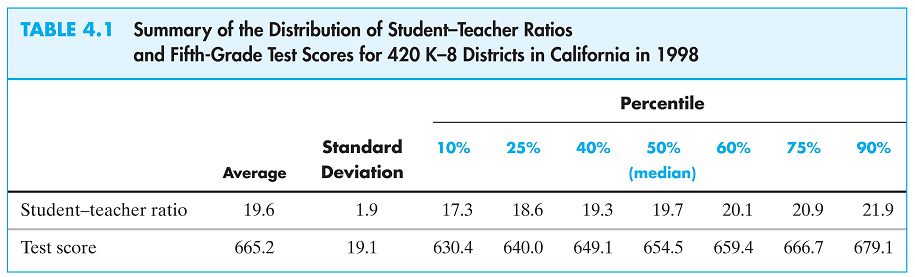
To estimate the model parameters of the class size/student performance model we have data from 420 California school districts in 1999
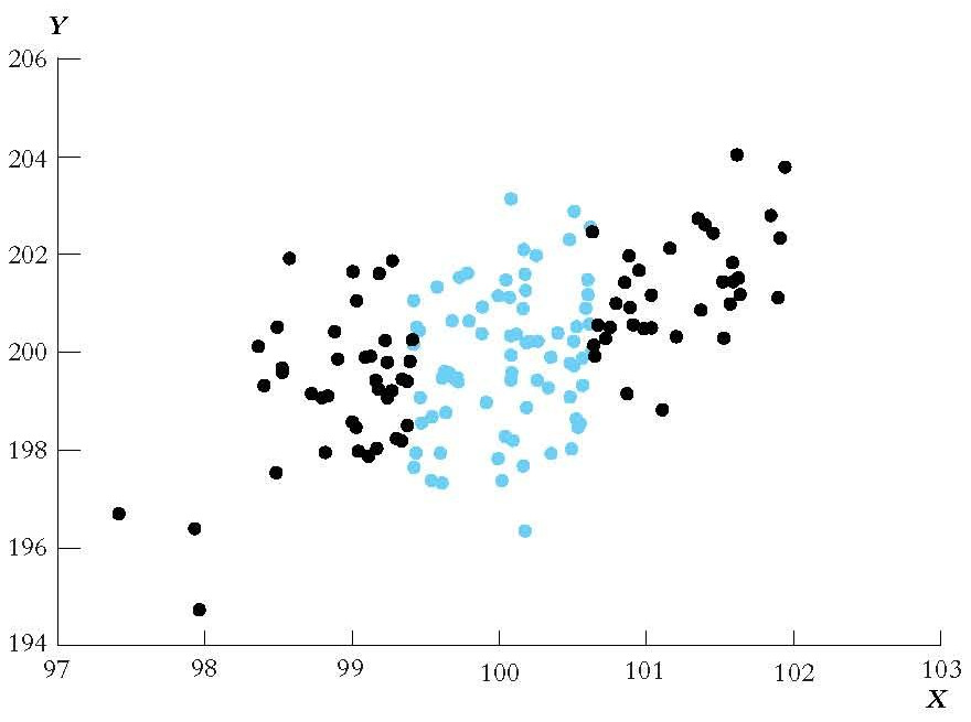
Correlation and Scatterplot
- The sample correlation is found to be -0.23, indicating a weak negative relationship.
- However, we need a better measure of causality
- We want to be able to draw a straight line through these dots characterizing the linear regression line, and from that we get the slope.
suppressPackageStartupMessages(library(AER,quietly=TRUE,warn.conflicts=FALSE))
library(ggplot2,quietly=TRUE,warn.conflicts=FALSE)
data("CASchools")
CASchools$str=CASchools$students/CASchools$teachers
CASchools$testscr=(CASchools$read+CASchools$math)/2
qplot(x=str, y=testscr, data=CASchools, geom="point",
      xlab="Student/Teacher Ratio", ylab="Test Scores")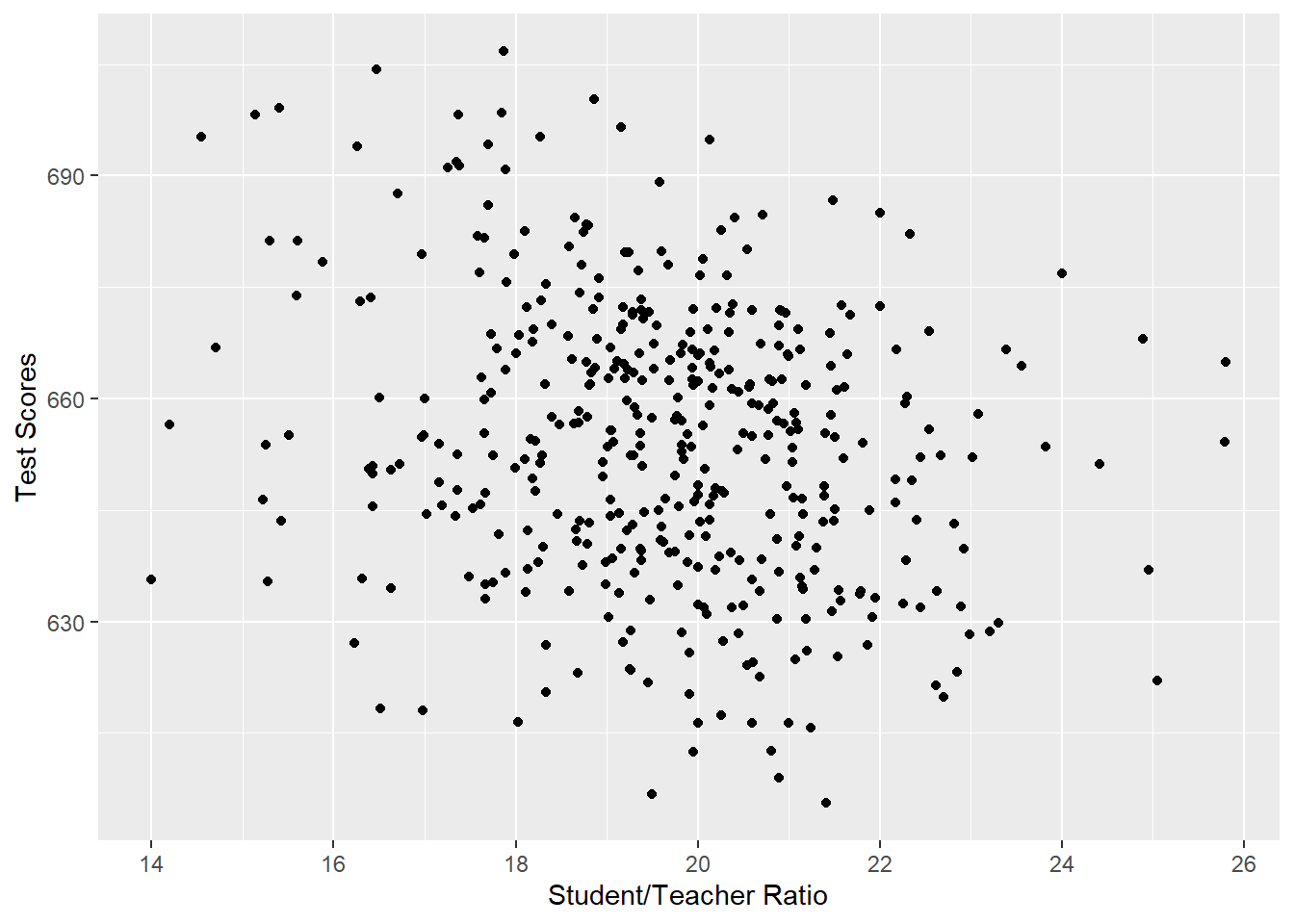
9.2 Estimators
You are already familiar with one estimator for a series, the mean.
Suppose you have n observations of \(y_i\). \[y_1,y_2,y_3,...,y_n\] If I have you guess the next value what would it be?
Let’s call this guess \(\hat{y}\)
The difference between \(y_i - \hat{y}=error= u_i\)
The error captures everything we do not know. It captures how far off our model is from the actual data. A good estimator minimizes the size of the error.
One way to capture the size of the error is to use the variance of the error.
\[\frac{1}{n}\sum_i^n (u_i-\bar{u})^2 = \frac{1}{n}\sum_i^n u_i^2=\frac{1}{n}\sum_i^n (y_i-\hat{y})^2\] Let’s assume that the mean of the errors is zero. How can we pick \(\hat{y}\) to make this sum as small as possible (minimization problem)?
We can solve for the minimum using calculus.
\[\frac{d}{d\hat{y}}\frac{1}{n}\sum_i^n (y_i-\hat{y})^2=\frac{-2}{n}\sum_i^n (y_i-\hat{y})=0 \\ \frac{1}{n}\sum_i^n (y_i-\hat{y})=0 \\ \frac{1}{n}\sum_i^n y_i-\hat{y}=\bar{y}-\hat{y}=0 \\ \bar{y} = \hat{y}\] For regression, we are essentially doing the same thing.
- The ordinary least squares (OLS) estimator selects estimates for the model parameters that minimize the distance between the sample regression line (function) and the observed data.
- Recall that we use \(\bar{Y}\) as an estimator of \(E[Y]\) since it minimizes \(\sum_i (Y_i - m)^2\)
- With OLS we are interested in minimizing \[\min_{b_0,b_1} \sum_i [Y_i - (b_0 + b_1 X_i)]^2\] We want to find \(b_0\) and \(b_1\) such that the mistakes between the observed \(Y_i\) and the predicted value \(b_0 + b_1 X_i\) are minimized.
See the appendix for the derivation
The OLS estimator of \(\beta_1\) is \[\hat{\beta}_1 = \frac{\sum_i (X_i - \bar{X})(Y_i - \bar{Y})}{\sum_i (X_i - \bar{X})^2} = \frac{s_{XY}}{s_X^2}\]
The OLS estimator of \(\beta_0\) is \[\hat{\beta}_0 = \bar{Y} - \hat{\beta}_1 \bar{X}\]
The predicted value of \(Y_i\) is \[\hat{Y}_i = \hat{\beta}_0 + \hat{\beta}_1 X_i\]
The error in predicting \(Y_i\) is called the residual \[\hat{u}_i = Y_i - \hat{Y}_i\]
9.3 OLS Regression of Test Scores on Student-Teacher Ratio
Using data from the 420 school districts an OLS regression is run to estimate the relationship between test score and teacher-student ratio (STR).
\[\widehat{TestScore} = 698.9 - 2.28 \times STR\]
where \(\widehat{TestScore}\) is the predicted value. (This is referred to as test scores regressed on STR)
qplot(x=str, y=testscr, data=CASchools, geom="point", xlab="Student/Teacher
      Ratio", ylab="Test Scores") + geom_abline(intercept=698.9, slope=-2.28,
                                                color='blue')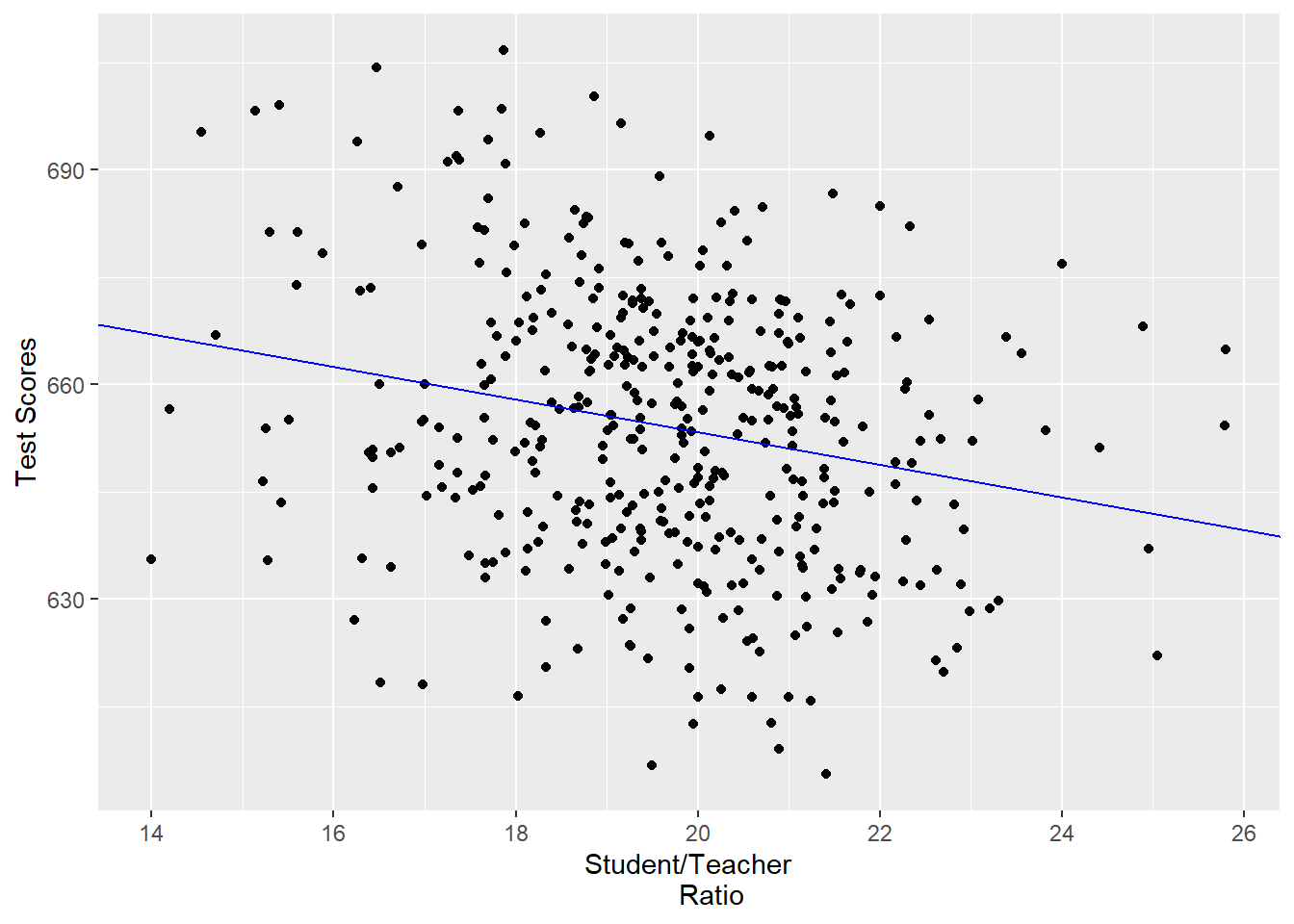
9.4 Goodness of Fit
Now that we’ve run an OLS regression we want to know
- How much does the regressor account for variation in the dependent variable?
- Are the observations tightly clustered around the regression line?
We have two useful measures
- The regression \(R^2\)
- The standard error of the regression \((SER)\)
9.4.1 The R Squared
The \(R^2\) is the fraction of the sample variance of \(Y_i\) (dependent variable) explained by \(X_i\) (regressor)
English Translation: \(R^2\) tells us how much of the variation in \(Y\) is explained by the variation in \(X\).
If \(R^2\) is equal 0.67, then the variation in \(X\) explain 67 percent of the variation in \(Y\). If \(R^2\)=1, then \(Y\) and \(X\) are perfectly colinear. \(X\) would predict \(Y\) perfectly. If \(R^2\)=0, then \(X\) and \(Y\) are independent. The regression line does no better than just using the mean of Y as your estimate.
- From the definition of the regression predicted value \(\hat{Y}_i\) we can write \[Y_i = \hat{Y}_i + \hat{u}_i\] and \(R^2\) is the ratio of the sample variance of \(\hat{Y}_i\) and the sample variance of \(Y_i\)
- \(R^2\) ranges from 0 to 1. \(R^2 = 0\) indicates that \(X_i\) has no explanatory power at all, while \(R^2 = 1\) indicates that it explains \(Y_i\) fully.
Let us define the total sum of squares \((TSS)\), the explained sum of squares \((ESS)\), and the sum of squared residuals \((SSR)\)
\[\begin{align*} Y_i &= \hat{Y}_i + \hat{u}_i \\ Y_i - \bar{Y} &= \hat{Y}_i - \bar{Y} + \hat{u}_i \\ (Y_i - \bar{Y})^2 &= (\hat{Y}_i - \bar{Y} + \hat{u}_i)^2 \\ (Y_i - \bar{Y})^2 &= (\hat{Y}_i - \bar{Y})^2 + (\hat{u}_i)^2 + 2(\hat{Y}_i - \bar{Y})\hat{u}_i \\ \underbrace{\sum_i(Y_i - \bar{Y})^2}_{TSS} &= \underbrace{\sum_i(\hat{Y}_i - \bar{Y})^2}_{ESS} + \underbrace{\sum_i(\hat{u}_i)^2}_{SSR} + \underbrace{2\sum_i(\hat{Y}_i - \bar{Y})\hat{u}_i}_{=0} \\ TSS &= ESS + SSR \end{align*}\]
\[TSS = ESS + SSR\]
\(R^2\) can be defined as \[R^2 = \frac{ESS}{TSS} = 1 - \frac{SSR}{TSS}\]
R-square - two warnings
Warning 1: Do not fall in love with \(R^2\)
R square is not necessarily the thing you are trying to maximize.
A GOOD R square really depends on the subject of your study.
When studying countries, especially in a time series setting, \(R^2 > 0.9\) is very common because a country tends to change slowly over time.
When studying states an \(0.8 > R^2 > 0.2\) usually observed.
When studying individual people an \(R^2 < .10\) is very common because people are very different and random.
Warning 2: Be careful about the abbreviations used when describing \(R^2\).
ESS = Explained Sum of Squares, but some books also use ESS as the Error Sum of Squares, which means the opposite.
RSS = Residual Sum of Squares, but some books use RSS as the Regression Sum of Squares, which means the opposite.
SSE = Sum of Squared Errors
SSR = Sum of Squared Regression
Confused yet
9.4.2 The Standard Error of the Regression
The standard error of the regression \((SER)\) is an estimator of the standard deviation of the population regression error \(u_i\).
We primarily use it to compare two regressions. The regression with the lower \(SER\) has a better fit.
Since we don’t observe \(u_1,\dots, u_n\) we need to estimate this standard deviation. We use \(\hat{u}_1,\dots, \hat{u}_n\) to calculate our estimate
\[SER = s_{\hat{u}}\] where \[s_{\hat{u}}^2 = \frac{1}{n-2}\sum_i \hat{u}_i^2 = \frac{SSR}{n-2}\]
9.4.3 Measure of Fit of Test Score on STR Regression
- The \(R^2\) is calculated to be 0.051. This means that the \(STR\) explains 5.1% of the variance in \(TestScore\).
- The \(SER\) is calculated to be 18.6. This is an estimate of the standard deviation of \(u_i\) which shows a large spread.
- Low \(R^2\) (or low \(SER\)) does not mean that the regression is bad: it means that there are other factors that have a strong influence on the dependent variable that have not been included in the regression.
9.5 Regression in R
Load the data
If you haven’t done so already, then let’s load the data into R. We want the CA Schools data from the AER library.
Enter the following code into R
- library(AER)
- data(CASchools)
Let’s Run a Regression
library(knitr)
library(modelsummary)
regress.results=lm(formula = testscr ~ str, data=CASchools)
modelsummary(regress.results, coef_rename = c(str="Student-Teacher Ratio"))
Modelsummary is a fantastic package for creating regression printouts. It has many features that allow you to customize your tables. Learn more about it at this .
9.6 The Least Squares Assumptions
- The error term \(u_i\) has a mean of zero, \(E[u_i]=0\).
- The error term is independent of the X’s, \(E[X_i u_i]=COV(X_i,u_i)=0\).
- The error term has a constant variance, \(Var[u_i|X_i]=\sigma^2\).
- The variables \(Y_i\) and \(X_i\) are independently identically distributed (i.e. they are a random sample)
- The relationship between \(Y_i\) and \(X_i\) is linear with respect to the parameters
- There are no large outliers.
- For testing reasons, we do assume the error terms are normally distributed.
These assumptions are necessary for us to be able to estimate, test, and interpret the \(\beta\)’s.
Let’s take a deeper dive on a few of these assumptions.
9.6.1 Assumption 1 and 2
\[E[u_i|X_i] = 0\]
- Other factors unaccounted for in the regression are unrelated to the regressor \(X_i\)
- While the dependent variable varies around the population regression line, on average the predicted value is correct
Two important take aways:
(1) there error has a mean of zero and (2) the error and X’s are independent.
9.6.2 Randomized Controlled Experiment
In a randomized controlled experiment, subjects are placed in treatment group \((X_i = 1)\) or the control group \((X_i = 0)\) randomly, not influenced by their unobservable characteristics, \(u_i\).
- Hence, \(E[u_i|X_i] = 0\).
Using observational data, \(X_i\) is not assigned randomly, therefore we must then think carefully about making assumption A.1.
9.6.3 Random Sample
For all \(i\), \((X_i, Y_i)\) are i.i.d.
- Since all observation pairs \((X_i, Y_i)\) are picked from the same population, then they are identically distributed.
- Since all observations are randomly picked, then they should be independent.
- The majority of data we will encounter will be i.i.d., except for data collected from the same entity over time (panel data, time series data)
Main takeaway: there should be no sample selection bias. The random sample should be a good representation of the population. Additionally, you want Y and X to be continuous throughout. For example an always positive number might not be represented well by a normal distribution.
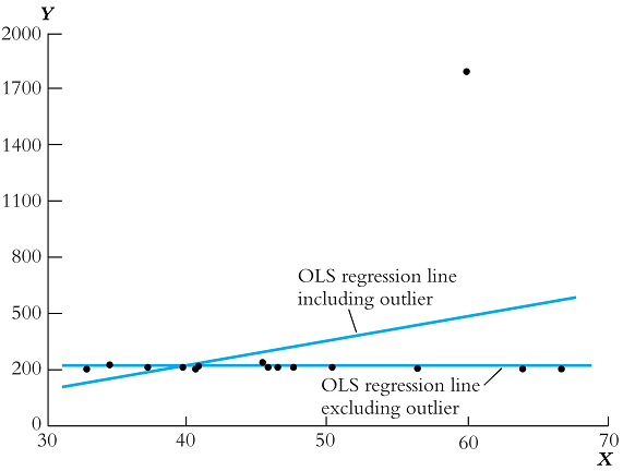
Assumption A.3: Large Outliers are Unlikely
\[0 < E[Y_i^4] < \infty\]
- None of the observed data should have extreme and “unexpected” values (larger than 3 standard deviations)
- Technically, this means that the fourth moment should be positive and finite
- You should look at your data (plot it) to see if any of the observations are suspicious, and then double check there was no error in the data.
9.7 Sometimes the relationship is not Linear
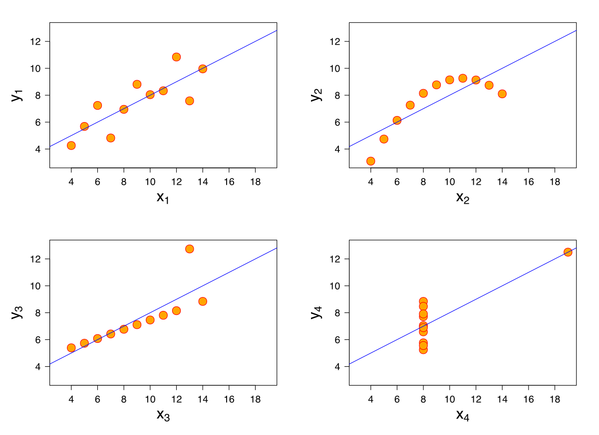 All of the above datasets produce the same regression, but it is clear from the scatter plots that the relationships are not the same. This example highlights the effects of outliers and functional form on our regression line.
We will show later on that linear regression can capture non-linear effects. Often people often confuse that the relationship between Y and X must be linear in order for you to use linear regression. The only part that needs to be linear are the parameters \((\beta's)\).
9.8 Sampling Distribution
Coefficients are Random Variables
- Since our regression coefficient estimates, \(\beta_0\) and \(\beta_1\), depend on a random sample \((X_i, Y_i)\) they are random variables
- While their distributions might be complicated for small samples, for large samples, using the Central Limit Theorem, they can be approximated by a normal distribution.
- It is important for us to have a way to describe their distribution, in order for us to carry out our inferences about the population.
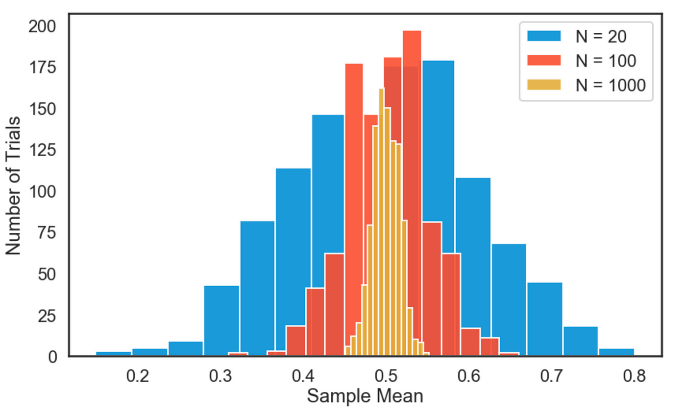
Review of Sampling Distribution of the Sample Mean of Y
When we have a large sample, we can approximate the distribution of the random variable \(\bar{Y}\) by a normal distribution with mean \(\mu_Y\).
The Sampling Distribution of the Model Coefficient Estimators
When the linear regression assumption hold, we can do the same thing with our parameter estimates.
- Both estimates are unbiased: \(E[\hat{\beta}_0] = \beta_0\) and \(E[\hat{\beta}_1] = \beta_1\).
- Using the same reasoning as we did with \(\bar{Y}\), we can use the CLT to argue that \(\hat{\beta}_0\) and \(\hat{\beta}_1\) are both approximately normal
- The sample variance of \(\hat{\beta}_1\) is \[\sigma_{\hat{\beta}_1}^2 = \frac{1}{n-1}\frac{Var(u_i)}{Var(X_i)}\]
- As the sample size increases, \(n\), \(\sigma_{\hat{\beta}_1}^2\) decreases to zero. This property is known as consistency. The OLS estimate of \(\hat{\beta}_1\) is said to be consistent. This is the reason people were so excited about BIG DATA.
- The larger \(Var(X_i)\) is (aka more variation in X), then the smaller is \(\sigma_{\hat{\beta}_1}^2\) and hence a tighter prediction of \(\beta_1\).
- The larger the variance of the error term is, the less precise our estimates are. There is more we do not know.
The Effect of Greater Variance in X
9.9 Multiple Regression
- In the previous chapter, we consider a simple model with only two parameters
- constant
- slope
- In this model, we used only one explanatory variable to predict the dependent variable.
9.10 What is Multiple Regression
Let’s say we are interested in the effects of education on wages. In reality, there are many factors affecting wages
- Education: Years of schooling, type of school, IQ
- Experience: Previous Position, Previous Company, Previous Responsibilities
- Occupation: Lawyer, Doctor, Engineer, Mathematician
- Discrimination: Sex, Age, Race, Health, or Nationality
- Location: New York City or Downtown Louisville
How do we control for each of these factors? What pays more 2 years in graduate school or 2 years of work experience?
Multiple Regression allows us to answer these questions.
- Identify the relative importance of each variable
- Which variables matter in the prediction of wages and which do not
- Identify the marginal effect of each variable on wages
\[wages_{i}=\beta_0+\beta_1Education_{i}+\beta_2Experience_{i}+e_{i}\]
- \(\beta_1\) tells us the effect 1 additional year of schooling has on your wages, holding your level of Experience constant
- \(\beta_2\) tells us the effect 1 additional year of work experience has on your wages, holding your level of Education constant
- \(\beta_0\) tells us your level of wages if you had no schooling and no work experience. (You can think of this as minimum wage)
- Note, each variable is index by (i), this index represent a specific person in our data set.
- The observed levels of education, experience, and wages changes with each person. The index give us a method to keep track of these changes.
Multiple Regression also helps you generalize the functional relationships between variables
Although, wage increases with experience it may do so at a decreasing rate Each additional year of experience increases your wage by less than the previous year. Example: Wages
\[wages_{i}=\beta_0+\beta_1Education_{i}+\beta_2Experience_{i}+\beta_3Experience^2_{i}+e_{i}\]
The relative increase in wages for an additional year of experience is given by the first partial derivative
\[\frac{\partial wages_i}{\partial Experience}=\beta_2+2\beta_3 *Experience\]
If \(\beta_3 <0\), then wages are increasing at a decreasing rate (and may eventually decrease altogether)
An example, suppose the regression equation stated
\[wages_{i}=4.25+2.50Education_{i}+3.5Experience_{i}-.25Experience^2_{i}+e_{i}\]
Then the marginal effect of experience on wages would be \[\frac{\partial wages_i}{\partial Experience}=3.5-.50 *Experience\] In this example, wages start to fall after the 7th year. How do I know?
If the derivative is zero, then wages are no longer increasing or decreasing, but if the derivative is negative, then wages are falling.
\[\frac{\partial wages_i}{\partial Experience}< 0 \implies 3.5-.50 *Experience<0\] Let’s solve \[ 3.5-.50 *Experience<0 \\ 3.5<.50 *Experience \\ 3.5/.50 < Experience \\ 7 < Experience\] Any value of experience greater than 7 will lead to a decrease in wages.
9.11 Omitted Variable Bias
Omitted Factors in the Test Score Regression
Recall that our regression model was
\[TestScore = \beta_0 + \beta_1 STR + u_i,~i=1,\dots,n\]
There are probably other factors that are characteristics of school districts that would influence test scores in addition to STR. For example
- teacher quality
- computer usage
- and other student characteristics such as family background
By not including them in the regression, they are implicitly included in the error term \(u_i\)
This is typically not a problem, unless these omitted factors influence an included regressor
Consider the percentage of English learners in a school district as an omitted variable. Suppose that
- districts with more English learners do worse on test scores
- districts with more English learners tend to have larger classes
CASchools$stratio <- with(CASchools, students/teachers)
CASchools$score <- with(CASchools, (math + read)/2)
cor(CASchools$english, CASchools$score)
## [1] -0.6441238## [1] 0.1876424- Unobservable fluctuations in the percentage of English learners would influence test scores and the student teacher ratio variable
- The regression will then incorrectly report that STR is causing the change in test scores
- Thus we would have a biased estimator of the effect of STR on test scores
An OLS estimator will have omitted variable bias (OVB) if
The omitted variable is correlated with an included regressor
The omitted variable is a determinant of the dependent variable
What OLS assumption does OVB violate?
It violates the OLS assumption A.1: \(E[u_i|X_i] = 0\).
As \(u_i\) and \(X_i\) are correlated due to \(u_i\)’s causal influence on \(X_i\), \(E[u_i|X_i] \neq 0\). This causes a bias in the estimator that does not vanish in very large samples.
9.12 Omitted Variable Bias - Math
Suppose the true model is given as \[y=\beta_0+\beta_1 x_1+\beta_2 x_2+u\] but we estimate \(\widetilde{y}=\widetilde{\beta_0} + \widetilde{\beta_1} x_1 + u\), then \[\widetilde{\beta}_1=\frac{\sum{(x_{i1}-\overline{x})y_i}}{\sum{(x_{i1}-\overline{x})^2}}\]
Recall the true model, \[y=\beta_0+\beta_1 x_1+\beta_2 x_2+u\]
The numerator in our estimate for \(\beta_1\) is \[\widetilde{\beta}_1=\frac{\sum{(x_{i1}-\overline{x})(\beta_0+\beta_1 x_{i1}+\beta_2 x_{i2}+u_i)}}{\sum{(x_{i1}-\overline{x})^2}} \\ =\frac{\beta_1\sum{(x_{i1}-\overline{x})^2}+\beta_2\sum{(x_{i1}-\overline{x})x_{i2}}+\sum{(x_{i1}-\overline{x})u_i}}{\sum{(x_{i1}-\overline{x})^2}} \\ = \beta_1+\beta_2 \frac{\sum{(x_{i1}-\overline{x})x_{i2}}}{\sum{(x_{i1}-\overline{x})^2}}+\frac{\sum{(x_{i1}-\overline{x})u_i}}{\sum{(x_{i1}-\overline{x})^2}}\]
If the \(E(u_i)=0\), then by taking expectations we find \[E(\widetilde{\beta}_1)=\beta_1+\beta_2 \frac{\sum{(x_{i1}-\overline{x})x_{i2}}}{\sum{(x_{i1}-\overline{x})^2}}\]
From here we see clearly the two conditions need for an Omitted Variable Bias
The omitted variable is correlated with an included regressor (i.e. \(\sum{(x_{i1}-\overline{x})x_{i2}})\neq 0\))
The omitted variable is a determinant of the dependent variable (i.e. \(\beta_2\neq 0\))
Summary of the Direction of Bias
| Signs | \(Corr(x_1,x_2)>0\) | \(Corr(x_1,x_2)<0\) |
|---|---|---|
| \(\beta_2>0\) | Positive Bias | Negative Bias |
| \(\beta_2<0\) | Negative Bias | Positive Bias |
Formula for the Omitted Variable Bias
Since there is a correlation between \(u_i\) and \(X_i\), \(Corr(X_i, u_i) = \rho_{Xu} \ne 0\)
The OLS estimator has the limit \[\hat{\beta}_1 \overset{p}{\longrightarrow} \beta_1 + \rho_{Xu}\frac{\sigma_u}{\sigma_X}\] which means that \(\hat{\beta}_1\) approaches the right hand value with increasing probability as the sample size grows.
- The OVB problem exists no matter the size of the sample.
- NO BIG DATA SOLUTION
- The larger \(\rho_{Xu}\) is the bigger the bias.
- The direction of bias depends on the sign of \(\rho_{Xu}\).
Addressing OVB by Dividing the Data into Groups
In a multiple regression model, we allow for more than one regressor.
This allows us to isolate the effect of a particular variable holding all others constant.
In other words, we can minimize the OVB by including variables in the regression equation that are important and potentially correlated with other regressors.
Solution 1 for OVB: if you can include the omitted variable into the regression, then it is no longer . . well omitted.
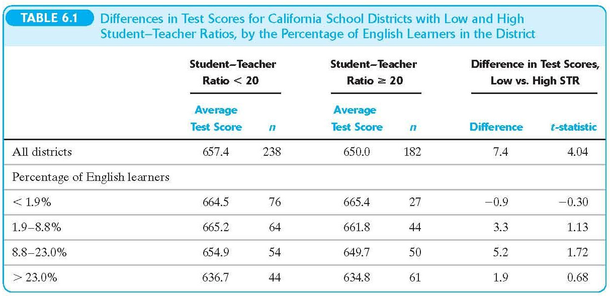
Look at what happens when we break down scores by Pct. English and Student-Teacher Ratio
 ## Simulation of OVB
# Simulated data
set.seed(123) # Set seed for reproducibility
n <- 10000 # Number of observations
p <- 0 # set correlation parameter
x1 <- rnorm(n)  # independent variable
x2 <- rnorm(n)+p*x1  # omitted variable
beta1 <- 1  # true coefficient for x1
beta2 <- 2  # true coefficient for x2
epsilon <- rnorm(n)  # error term
y <- 1 + beta1*x1 + beta2*x2 + epsilon  # dependent variable
lm_perfect <-lm(y~x1+x2)
# Model with the omitted variable
lm_omitted <- lm(y ~ x1)
# Model without the omitted variable
p <- 0.5
x2 <- rnorm(n)+p*x1  # independent variable
y <- 1 + beta1*x1 + beta2*x2 + epsilon  # dependent variable
lm_omitted2 <- lm(y ~ x1)
# Model with the omitted variable
p<- -0.5
x2 <- rnorm(n)+p*x1  # independent variable
y <- 1 + beta1*x1 + beta2*x2 + epsilon  # dependent variable
lm_omitted3 <- lm(y ~ x1) # Model with the omitted variable
lm_no_omitted <- lm(y ~ x1+x2)
modelsummary(list("Truth"=lm_perfect,"p=0"=lm_omitted,"p=0.5"=lm_omitted2,"p=-0.5"=lm_omitted3,"Both"=lm_no_omitted), gof_map = c("r.squared","nobs"))| Truth | p=0 | p=0.5 | p=-0.5 | Both | |
|---|---|---|---|---|---|
| (Intercept) | 0.993 | 0.975 | 0.982 | 1.023 | 0.993 |
| (0.010) | (0.022) | (0.022) | (0.022) | (0.010) | |
| x1 | 1.020 | 1.032 | 1.984 | 0.032 | 1.022 |
| (0.010) | (0.022) | (0.022) | (0.022) | (0.011) | |
| x2 | 1.997 | 2.004 | |||
| (0.010) | (0.010) | ||||
| R2 | 0.835 | 0.175 | 0.444 | 0.000 | 0.801 |
| Num.Obs. | 10000 | 10000 | 10000 | 10000 | 10000 |
9.14 Multiple Regression Model
Regressing On More Than One Variable
In a multiple regression model we allow for more than one regressor.
This allows us to isolate the effect of a particular variable holding all others constant.
The Population Multiple Regression Line
The population regression line (function) with two regressors would be
\[E[Y_i|X_{1i} = x_1, X_{2i} = x_2] = \beta_0 + \beta_1 x_1 + \beta_2 x_2\]
- \(\beta_0\) is the intercept
- \(\beta_1\) is the slope coefficient of \(X_{1i}\)
- \(\beta_2\) is the slope coefficient of \(X_{2i}\)
Interpretation of The Slope Coefficient
We interpret \(\beta_1\) (also referred to as the coefficient on \(X_{1i}\)), as the effect on \(Y\) of a unit change in \(X_1\), holding \(X_2\) constant or controlling for \(X_2\).
For simplicity let us write the population regression line as
\[Y = \beta_0 + \beta_1 X_1 + \beta_2 X_2\]
Suppose we change \(X_1\) by an amount \(\Delta X_1\), which would cause \(Y\) to change to \(Y + \Delta Y\).
\[Y + \Delta Y = \beta_0 + \beta_1 (X_1 + \Delta X_1) + \beta_2 X_2\]
\[Y = \beta_0 + \beta_1 X_1 + \beta_2 X_2 \\ Y + \Delta Y = \beta_0 + \beta_1 (X_1 + \Delta X_1) + \beta_2 X_2\]
Subtract the first equation from the second equation, yielding \[\begin{align*} \Delta Y &= \beta_1 \Delta X_1 \\ \beta_1 &= \frac{\Delta Y}{\Delta X_1} \end{align*}\]
\(\beta_1\) is also referred to as the partial effect on \(Y\) of \(X_1\), holding \(X_2\) fixed.
The same as with the single regressor case, the regression line describes the average value of the dependent variable and its relationship with the model regressors.
In reality, the actual population values of \(Y\) will not be exactly on the regression line since there are many other factors that are not accounted for in the model.
These other unobserved factors are captured by the error term \(u_i\) in the population multiple regression \[Y_i = \beta_0 + \beta_1 X_{1i} + \beta_2 X_{2i} + \cdots + \beta_k X_{ki} + u_i,~i=1,\dots,n\]
(Generally, we can have any number of k regressors as shown above)
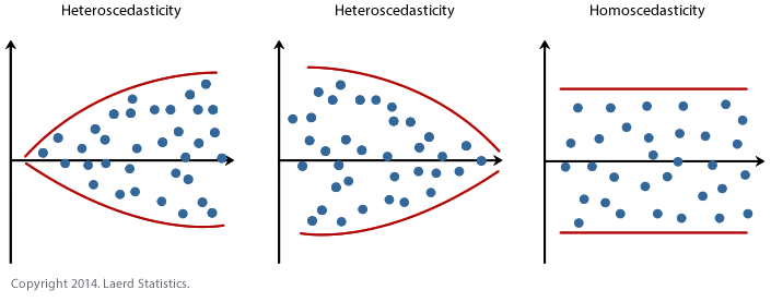
9.15 Homoscedasticity and Heteroskedasticity
As with the case of a single regressor model, the population multiple regression model can be either homoscedastic or heteroskedastic.
It is homoscedastic if
\[Var(u_i|X_{1i},\dots,X_{ki})\]
is constant for all \(i=1,\dots,n\). Otherwise, it is heteroskedastic.
In most cases (read virtually always), you will have heteroskedastic errors.
Visual of homoscedasticity and Heteroskedasticity
More on Heteroskedasticity
food <- read.csv("http://www.principlesofeconometrics.com/poe5/data/csv/food.csv")
food.ols <- lm(food_exp ~ income, data = food)
food$resi <- food.ols$residuals
library(ggplot2)
ggplot(data = food, aes(y = resi, x = income)) + geom_point(col = 'blue') + geom_abline(slope = 0)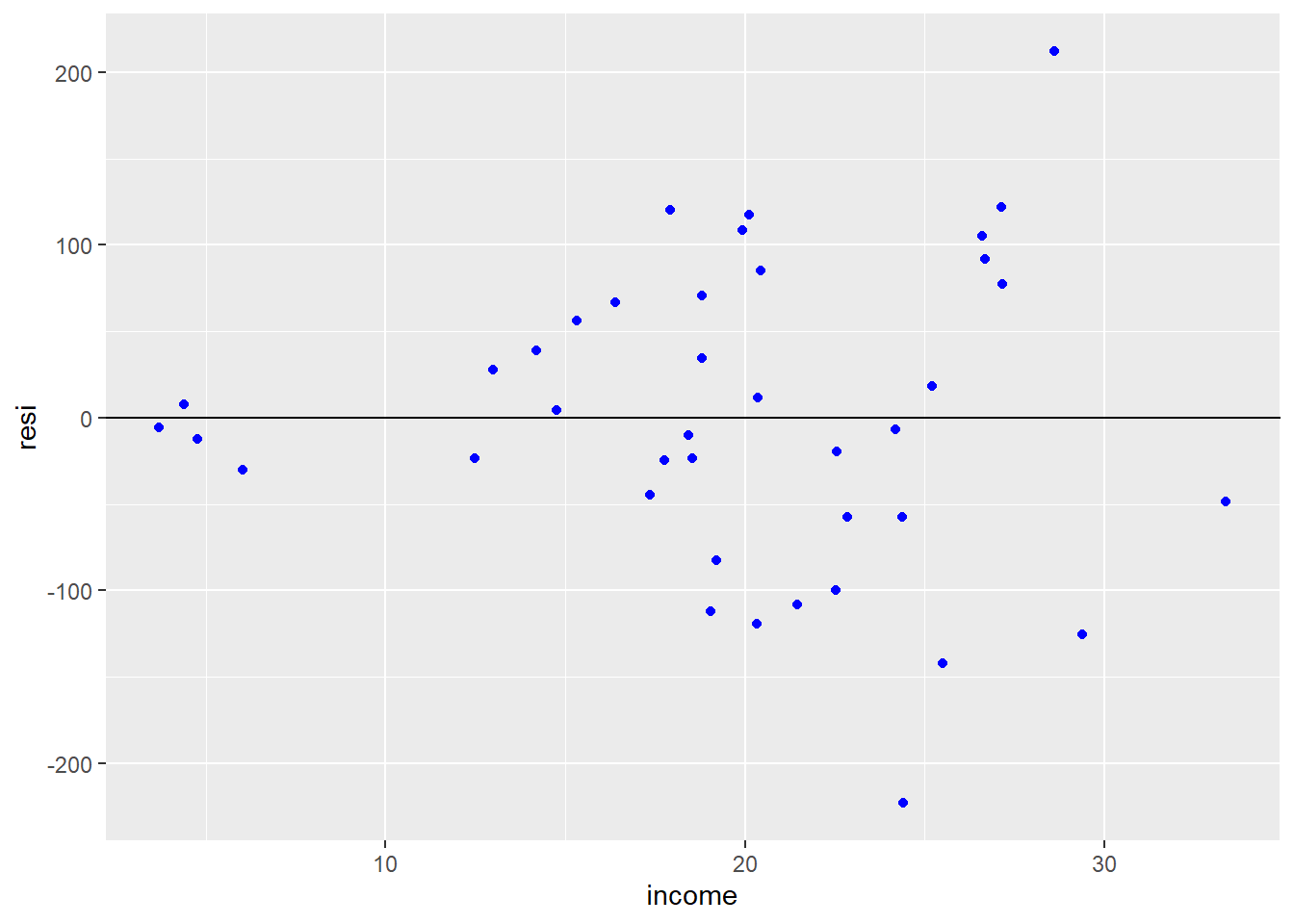
Two ways to test
First way to test is to check if the squared residuals are actually dependent of the variables.
\[e^2_i = \beta_0 + \beta_1*income_i\] The coefficient \(\beta_2\) should equal zero if the errors are homoscedastic.
##
## Call:
## lm(formula = resi^2 ~ income, data = food)
##
## Residuals:
##    Min     1Q Median     3Q    Max
## -14654  -5990  -1426   2811  38843
##
## Coefficients:
##             Estimate Std. Error t value Pr(>|t|)
## (Intercept)  -5762.4     4823.5  -1.195  0.23963
## income         682.2      232.6   2.933  0.00566 **
## ---
## Signif. codes:  0 '***' 0.001 '**' 0.01 '*' 0.05 '.' 0.1 ' ' 1
##
## Residual standard error: 9947 on 38 degrees of freedom
## Multiple R-squared:  0.1846, Adjusted R-squared:  0.1632
## F-statistic: 8.604 on 1 and 38 DF,  p-value: 0.005659
Option 2 The Breusch-Pagan Test
##
##  studentized Breusch-Pagan test
##
## data:  food.ols
## BP = 7.3844, df = 1, p-value = 0.006579
Again we find evidence of Heteroskedasticity
How to correct for Heteroskedasticity
There are three ways to correct for heteroskedasticity.
- The packages
lmtestandsandwichcan correct your standard errors after running the regression. - The package
fixestcan run robust standard errors using the functionfeols. - The package
estimaterhas a function calledlm_robust, which works with the same syntax haslm. - The package
modelsummarycan correct for robust standard errors as well.
| IID SE | Robust SE | |
|---|---|---|
| (Intercept) | 83.416 | 83.416 |
| (43.410) | (27.464) | |
| income | 10.210 | 10.210 |
| (2.093) | (1.809) | |
| Num.Obs. | 40 | 40 |
| R2 | 0.385 | 0.385 |
| R2 Adj. | 0.369 | 0.369 |
| AIC | 477.0 | 477.0 |
| BIC | 482.1 | 482.1 |
| Log.Lik. | -235.509 | -235.509 |
| F | 23.789 | 31.850 |
| RMSE | 87.25 | 87.25 |
| Std.Errors | IID | HC1 |
We can see from the table that the coefficients are exactly the same, but the standard errors are very different.
9.16 The OLS Estimator
Similar to the single regressor case, we do not observe the true population parameters \(\beta_0,\dots,\beta_k\). From an observed sample \(\{(Y_i, X_{1i},\dots,X_{ki})\}_{i=1}^n\) we want to calculate an estimator of the population parameters
We do this by minimizing the sum of squared differences between the observed dependent variable and its predicted value
\[\min_{b_0,\dots,b_k} \sum_i (Y_i - b_0 - b_1 X_{1i} - \cdots - b_k X_{ki})^2\]
Similar to the simple linear regression case, we would have k+1 equations and k+1 unknowns.
Let the multiple regression equation be represented by \[Y=X\beta+u\]
where we observe n observations, a dependent variable \(Y\) is a nx1 vector, X is a nxk matrix of k difference explanatory variables, \(u\) is the error term, which is assumed to have a mean of zero and a finite variance.
We are interested in estimating the parameter \(\beta\), which is a kx1 vector.
Our most important assumption is that \(E[X'u]=0\). If so, then we can write the moment condition as \[\begin{align*} X'u &= 0 \\X'(Y-X\beta) &=0 \\ X'Y &= X'X\beta \\ (X'X)^{-1}X'Y &= \beta \end{align*}\]
where \((X'X)^{-1}\) is the covariance matrix of X and X’Y is the covariance of X and Y. Notice this is exactly like the simple linear case, where our slope estimator is the COV(X,Y)/VAR(X)
The resulting estimators are called the ordinary least squares (OLS) estimators: \(\hat{\beta}_0,\hat{\beta}_1,\dots,\hat{\beta}_k\)
The predicted values would be
\[\hat{Y}_i = \hat{\beta}_0 + \hat{\beta}_1 X_{1i} + \cdots + \hat{\beta}_k X_{ki},~i=1,\dots,n\]
The OLS residuals would be
\[\hat{u}_i = Y_i - \hat{Y}_i,~i=1,\dots, n\]
9.17 Application to Test Scores and the STR
Recall that, using observations from 420 school districts, we regressed student test scores on STR we got \[\widehat{TestScore} = 698.9 - 2.28 \times STR\]
However, there was concern about the possibility of OVB due to the exclusion of the percentage of English learners in a district, when it influences both test scores and STR.
We can now address this concern by including the percentage of English learners in our model
\[ TestScore_i = \beta_0 + \beta_1 \times STR_i + \beta_2 \times PctEL_i + u_i \]
where \(PctEL_i\) is the percentage of English learners in school district \(i\).
(Notice that we are using heteroskedastic-robust standard errors)
regress.results <- lm(score ~ stratio + english, data = CASchools)
het.se <- vcovHC(regress.results)
coeftest(regress.results, vcov.=het.se)
##
## t test of coefficients:
##
## Estimate Std. Error t value Pr(>|t|)
## (Intercept) 686.032245 8.812242 77.8499 < 2e-16 ***
## stratio -1.101296 0.437066 -2.5197 0.01212 *
## english -0.649777 0.031297 -20.7617 < 2e-16 ***
## ---
## Signif. codes: 0 '***' 0.001 '**' 0.01 '*' 0.05 '.' 0.1 ' ' 1Comparing Estimates
In the single regressor case our estimates were \[\widehat{TestScore} = 698.9 - 2.28 \times STR\] and with the added regressor we have \[\widehat{TestScore} = 686.0 - 1.10 \times STR - 0.65 \times PctEL\]
Notice the lower effect of STR in the second regression.
The second regression captures the effect of STR holding the percentage of English learners constant. We can conclude that the first regression does suffer from OVB. This multiple regression approach is superior to the tabular approach shown before; we can give a clear estimate of the effect of STR and it is possible to easily add more regressors if the need arises.
9.18 Measures of Fit
9.18.1 The Standard Error of the Regression (SER)
Similar to the single regressor case, except for the modified adjustment for the degrees of freedom, the \(SER\) is
\[SER = s_{\hat{u}}\text{ where }s_{\hat{u}}^2 = \frac{\sum_i \hat{u}^2_i}{n - k - 1} = \frac{SSR}{n - k - 1}\]
Instead of adjusting for the two degrees of freedom used to estimate two coefficients, we now need to adjust for \(k+1\) estimations.
9.18.2 The R Squared
\[ R^2 = \frac{EES}{TSS} = 1 - \frac{SSR}{TSS} \]
- Since OLS estimation is a minimization of \(SSR\) problem, every time a new regressor is added to a regression, the \(R^2\) would be nondecreasing.
- This does not correctly evaluate the explanatory power of adding regressors-it tends to inflate it
9.18.3 The Adjusted R Squared
In order to address the inflation problem of the \(R^2\) we can calculated an “adjusted” version to corrects for that \[\bar{R}^2 = 1 - \frac{n-1}{n-k-1}\frac{SSR}{TSS} = 1 - \frac{s_{\hat{u}}^2}{s_Y^2}\]
The factor \(\frac{n-1}{n-k-1}\) is always \(> 1\), and therefore we always have \(\bar{R}^2 < R^2\).
When a regressor is added, it has two effects on \(\bar{R}^2\)
- The Sum of Squared Residuals, \(SSR\), decreases
- \(\frac{n-1}{n-k-1}\) increases, “adjusting” for the inflation effect
It is possible to have \(\bar{R}^2 < 0\)
From our multiple regression of the test scores on STR and the percentage of English learners we have the \(R^2\), \(\bar{R}^2\), and \(SER\)
## [1] 0.4264315## [1] 0.4236805## [1] 14.46448We notice a large increase in the \(R^2 = 0.426\) compared to that of the single regressor estimation 0.051. Adding the percentage of English learners has added a significant increase in the explanatory power of the regression.
Because \(n\) is large compared to the two regressors used, \(\bar{R}^2\) is not very different from \(R^2\).
We must be careful not to let the increase in \(R^2\) (or \(\bar{R}^2\)) drive our choice of regressors.
9.19 The Least Squares Assumptions in Multiple Regression
For multiple regressions we have four assumptions: three of them are updated versions of the single regressor assumptions and one new assumption.
- A.1: The conditional distribution of \(u_i\) given \(X_{1i},\dots,X_{ki}\) has a mean of zero \(E[u_i|X_{1i},\dots,X_{ki}] = 0\)
- A.2: \(\forall i, (X_{1i}, \dots, X_{ki}, Y_i)\) are i.i.d.
- A.3: Large outliers are unlikely
Assumption A.4: No Perfect Multicollinearity (1)
The regressors exhibit perfect multicollinearity if one of the regressors is a linear function of the other regressor.
Assumption A.4 requires that there be no perfect multicollinearity
Perfect multicollinearity can occur if a regressor is accidentally repeated, for example, if we regress \(TestScore\) on \(STR\) and \(STR\) again (R simply ignores the repeated regressor).
This could also occur if a regressor is a multiple of another.
Assumption A.4: No Perfect Multicollinearity (2)
Mathematically, this is not allowed because it leads to division by zero.
Intuitively, we cannot logically think of measuring the effect of \(STR\) while holding other regressors constant since the other regressor is \(STR\) as well (or a multiple of)
Examples of Perfect Multicollinearity
Fraction of English learners
“Not very small” classes:
Let \(NVS_i = 1 \) if \( STR_i \geq 12\)
None of the data available has \(STR_i \le 12 \) therefore \( NVS_i\) is always equal to \(1\).
Example 2: The Dummy Variable Trap
Suppose we want to categorize school districts as rural, suburban, and urban
- We use three dummy variables \(Rural_i\), \(Suburban_i\), and \(Urban_i\)
- If we included all three dummy variables in our regress we would have perfect multicollinearity: \(Rural_i + Suburban_i + Urban_i = 1\) for all \(i\)
- Generally, if we have \(G\) binary variables and each observation falls into one and only one category we must eliminate one of them: we only use \(G-1\) dummy variables
9.20 Imperfect Multicollinearity
Imperfect multicollinearity means that two or more regressors are highly correlated. It differs from perfect multicollinearity it that they don’t have to be exact linear functions of each other.
- For example, consider regressing \(TestScore\) on \(STR\), \(PctEL\) (the percentage of English learners), and a third regressor that is the percentage of first-generation immigrants in the district.
- There will be strong correlation between \(PctEL\) and the percentage of first-generation immigrants
- Sample data will not be very informative about what happens when we change \(PctEL\) holding other regressors fixed
- Imperfect multicollinearity does not pose any problems to the theory of OLS estimation + OLS estimators will remain unbiased. + However, the variance of the coefficient on correlated regressors will be larger than if they were uncorrelated.
The tell-tale sign of multicolinearity is when you include two highly correlated variables together in the same regression. You notice that neither variable is statistically significant. You drop one of the variables and immediately the remaining variable becomes highly significant. You switch the variables and you run them again. Again, you find the included variable is highly significant. Just to be sure, you run the regression again with both variables and now neither variable is significant.
9.20.1 Multicolinearity R Example
# Load necessary libraries
library(tidyverse)

# Simulate correlated independent variables
set.seed(123)
n <- 100 # Number of observations
x1 <- rnorm(n, mean = 10, sd = 2) # Independent variable 1
x2 <- x1 + rnorm(n, mean = 0, sd = .51) # Independent variable 2 (highly correlated with x1)

# Generate dependent variable with some noise
y <- 2 * x1 + 2* x2 + rnorm(n, mean = 0, sd = 6)

# Create a data frame
data <- data.frame(x1, x2, y)

# Check the correlation between x1 and x2
correlation <- cor(data[, c("x1", "x2")])
print(correlation)
## x1 x2
## x1 1.0000000 0.9645841
## x2 0.9645841 1.0000000# Fit a linear regression model
model <- lm(y ~ x1 + x2, data = data)
model2 <- lm(y ~ x1, data = data)
model3<- lm(y ~ x2, data = data)
# Print the summary of the regression model
modelsummary::modelsummary(list(model, model2, model3))| (1) | (2) | (3) | |
|---|---|---|---|
| (Intercept) | 4.806 | 4.991 | 5.639 |
| (3.251) | (3.296) | (3.166) | |
| x1 | 1.320 | 3.570 | |
| (1.191) | (0.319) | ||
| x2 | 2.280 | 3.525 | |
| (1.165) | (0.308) | ||
| Num.Obs. | 100 | 100 | 100 |
| R2 | 0.578 | 0.561 | 0.573 |
| R2 Adj. | 0.569 | 0.557 | 0.568 |
| AIC | 637.1 | 639.0 | 636.4 |
| BIC | 647.5 | 646.8 | 644.2 |
| Log.Lik. | -314.554 | -316.492 | -315.183 |
| F | 66.456 | 125.453 | 131.377 |
| RMSE | 5.62 | 5.73 | 5.66 |
Logic: When two variables are highly co-linear it means they overlap a great deal. Therefore, if you include both variables in the same regression, how much additional information are you gaining from including both variables instead of just one
The Variance Inflation Factor (VIF) is a measure used to detect multicollinearity in a regression model. It assesses how much the variance of an estimated regression coefficient is increased due to multicollinearity. A VIF value greater than 1 indicates some level of multicollinearity. A VIF value between 1 and 5 indicates some correlation, but not severe enough to require attention. A higher VIF value suggest stronger multicollinearity and may cause your statistics to become unreliable. Here’s how to calculate the VIF and incorporate it into the previous example:
# Calculate Variance Inflation Factor (VIF)
vif_data <- data.frame(variables = colnames(data[, c("x1", "x2")]),
                       vif = round(vif(model), 2))

print(vif_data)
## variables vif
## x1 x1 14.37
## x2 x2 14.37You can practice some more using VIF with this module
There are two advanced solutions to multicolinearity, ridge regression and lasso regression. I will add chapters later about these two models. In the meantime, I suggest the following websites for explanations.
9.21 The Distribution of the OLS Estimators in Multiple Regression
- Since our OLS estimates depend on the sample, and we rely on random sampling, there will be uncertainty about how close these estimates are to the true model parameters
- We represent this uncertainty by a sampling distribution of \(\hat{\beta}_0, \hat{\beta}_1,\dots,\hat{\beta}_k\)
- The estimators \(\hat{\beta}_0, \hat{\beta}_1,\dots,\hat{\beta}_k\) are unbiased and consistent
- In large samples, the joint sampling distribution of the estimators is well approximated by a multivariate normal distribution, where each \(\hat{\beta}_j \sim N(\beta_j, \sigma_{\hat{\beta}_j}^2)\)
9.22 Dummy Variables
Dummy Variables are not dumb at all. Dummy (binary) Variables allows us to capture information from non-numeric or non-continuous variables.
We can control for observable categories such as race, religion, gender, and state of residence. These variables are very powerful in capturing unobserved characteristics of people, places, and things.
For example, it may be hard to capture the culture or topography of certain place. These things could affect a persons behavior. If you live in very cold climates, then you may be less likely to spend time outside. This is valuable information to include in your regression, but it could be difficult to control for using conventional continuous variables.
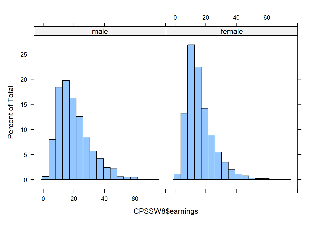
Current Population Survey (CPS) is produced by the BLS and provides data on labor force characteristics of the population, including the level of employment, unemployment, and earnings.
- 65,000 randomly selected U.S. households are surveyed each month.
- The MARCH survey is more detailed than in other months and asks questions about earnings during the previous year.
| Variables | Definition |
|---|---|
| gender | 1 if female; 0 if male |
| Age | Age in Years |
| earnings | Avg. Hourly Earnings |
| education | Years of Education |
| Northeast | 1 if from the Northeast, 0 otherwise |
| Midwest | 1 if from the Midwest, 0 otherwise |
| South | 1 if from the South, 0 otherwise |
| West | 1 if from the West, 0 otherwise |
library("AER")
library("lattice")
data("CPSSW8")
modelsummary::datasummary_balance(~1,data = CPSSW8, output = "html")| Mean | Std. Dev. | ||
|---|---|---|---|
| earnings | 18.4 | 10.1 | |
| age | 41.2 | 10.6 | |
| education | 13.6 | 2.5 | |
| N | Pct. | ||
| gender | male | 34348 | 55.9 |
| female | 27047 | 44.1 | |
| region | Northeast | 12371 | 20.1 |
| Midwest | 15136 | 24.7 | |
| South | 18963 | 30.9 | |
| West | 14925 | 24.3 |
| male (N=34348) | female (N=27047) | ||||||
|---|---|---|---|---|---|---|---|
| Mean | Std. Dev. | Mean | Std. Dev. | Diff. in Means | Std. Error | ||
| earnings | 20.1 | 10.6 | 16.3 | 9.0 | −3.7 | 0.1 | |
| age | 41.0 | 10.6 | 41.5 | 10.6 | 0.5 | 0.1 | |
| education | 13.5 | 2.5 | 13.8 | 2.4 | 0.2 | 0.0 | |
| N | Pct. | N | Pct. | ||||
| region | Northeast | 6898 | 20.1 | 5473 | 20.2 | ||
| Midwest | 8505 | 24.8 | 6631 | 24.5 | |||
| South | 10305 | 30.0 | 8658 | 32.0 | |||
| West | 8640 | 25.2 | 6285 | 23.2 | |||
Statistical discrimination
One thing we can do with categorical variables is to identify statistical discrimination.
A simple linear regression of Avg. Hourly Earnings on Gender will give us a quick comparison of earnings between females and males.
| (1) | |
|---|---|
| (Intercept) | 20.086 |
| (0.054) | |
| Female | -3.748 |
| (0.081) | |
| Num.Obs. | 61395 |
| R2 | 0.034 |
Let’s add some controls
In this second regression we include some additional explanatory variables.
\[earnings_i = \beta_0+\beta_1 Female_i +\beta_2 age + \beta_3 education\]
| earnings | ||
| (1) | (2) | |
| Female | -3.748c (0.081) | -4.250c (0.071) |
| Age | 0.157c (0.003) | |
| Education | 1.748c (0.014) | |
| Constant | 20.086c (0.054) | -10.026c (0.237) |
| N | 61,395 | 61,395 |
| R2 | 0.034 | 0.249 |
| Adjusted R2 | 0.034 | 0.249 |
| Notes: | ***Significant at the 1 percent level. | |
| **Significant at the 5 percent level. | ||
| *Significant at the 10 percent level. | ||
Warning about Statistical Discrimination Although, we estimate that women earn less than men. It would be incorrect to say that this definitely proves women earn less than men do to discrimination.
- The dummy variable does not take on all the attributes of the group. It simply labels them
- There could still be difference in amount of education, type of education, amount of experience, age, race, etc.
- All of these could be contributing to the differences between the genders, but since we are not controlling for them it appears as if there is gender discrimination.
- This problem is even worse for race.
- See a large twitter fight about the subject here amoung economists
- Summary if you think there is systemic racism then the amount of education receive will not be independent of the error term.
9.23 Quadratic function
Economic theory tells us that there are diminishing returns to productivity. As we age we become more productivity, but at a decreasing rate. One way to account for this change is by including a quadratic term in our specification.
\[earnings_i = \beta_0+\beta_1 Female_i +\beta_2 age + \beta_3 age^2 +\beta_4 education\]
CPSSW8$age2=CPSSW8$age*CPSSW8$age
m3 = lm(earnings ~ factor(gender)+age+age2+education, data=CPSSW8)
stargazer::stargazer(m1,m2,m3,type="html",omit.stat = c("f","ser"), covariate.labels = c("Female","Age","Age Sq","Education"), star.char = c("a","b","c"))| earnings | |||
| (1) | (2) | (3) | |
| Female | -3.748c (0.081) | -4.250c (0.071) | -4.239c (0.071) |
| Age | 0.157c (0.003) | 0.986c (0.025) | |
| Age Sq | -0.010c (0.0003) | ||
| Education | 1.748c (0.014) | 1.724c (0.014) | |
| Constant | 20.086c (0.054) | -10.026c (0.237) | -25.762c (0.522) |
| N | 61,395 | 61,395 | 61,395 |
| R2 | 0.034 | 0.249 | 0.262 |
| Adjusted R2 | 0.034 | 0.249 | 0.262 |
| Notes: | ***Significant at the 1 percent level. | ||
| **Significant at the 5 percent level. | |||
| *Significant at the 10 percent level. | |||
9.24 Interaction term
Potentially, the returns from education are different by gender. We add this feature to the model by including an interaction term. We multiply gender and education.
\[earnings_i = \beta_0+\beta_1 Female_i +\beta_2 age+ \beta_3 age^2 \\ +\beta_4 education+ \beta_5 education *Female\]
We see from the regression results that there are not much difference with respect to education
| earnings | ||||
| (1) | (2) | (3) | (4) | |
| Female | -3.748c (0.081) | -4.250c (0.071) | -4.239c (0.071) | -4.847c (0.405) |
| Female*Educ | 0.044 (0.029) | |||
| Age | 0.157c (0.003) | 0.986c (0.025) | 0.986c (0.025) | |
| Age Sq | -0.010c (0.0003) | -0.010c (0.0003) | ||
| Education | 1.748c (0.014) | 1.724c (0.014) | 1.706c (0.019) | |
| Constant | 20.086c (0.054) | -10.026c (0.237) | -25.762c (0.522) | -25.529c (0.544) |
| N | 61,395 | 61,395 | 61,395 | 61,395 |
| R2 | 0.034 | 0.249 | 0.262 | 0.262 |
| Adjusted R2 | 0.034 | 0.249 | 0.262 | 0.262 |
| Notes: | ***Significant at the 1 percent level. | |||
| **Significant at the 5 percent level. | ||||
| *Significant at the 10 percent level. | ||||
9.25 Location, Location, Location
There are often unobservable characteristics about markets that we would like to capture, but we just don’t have this variable (i.e. unemployment rate by gender or sector, culture, laws, etc).
One way to handle this problem is to use categorical variables for the location of the person or firm.
These categorical variables will capture any time invariant differences between locations.
| earnings | |||
| (1) | (2) | (3) | |
| Female | -4.239c (0.071) | -4.847c (0.405) | -4.797c (0.404) |
| MidWest | -1.257c (0.105) | ||
| South | -1.217c (0.101) | ||
| West | -0.425c (0.106) | ||
| Education*Female | 0.044 (0.029) | 0.042 (0.029) | |
| Age | 0.986c (0.025) | 0.986c (0.025) | 0.983c (0.025) |
| Age Squared | -0.010c (0.0003) | -0.010c (0.0003) | -0.010c (0.0003) |
| Education | 1.724c (0.014) | 1.706c (0.019) | 1.701c (0.019) |
| Constant | -25.762c (0.522) | -25.529c (0.544) | -24.603c (0.550) |
| N | 61,395 | 61,395 | 61,395 |
| R2 | 0.262 | 0.262 | 0.265 |
| Adjusted R2 | 0.262 | 0.262 | 0.265 |
| Notes: | ***Significant at the 1 percent level. | ||
| **Significant at the 5 percent level. | |||
| *Significant at the 10 percent level. | |||
9.26 Log Transformation
The normality assumption about the error term implies the dependent variable can potentially take on both negative and positive values.
However, there are some variables we use often that are always positive
- price
- quantity
- income
- wages
One method used to insure that we have a positive dependent variable is to transform the dependent variable by taking the natural log.
| earnings | log(earnings) | ||
| (1) | (2) | (3) | |
| Female | 0.986c (0.025) | 0.983c (0.025) | 0.062c (0.001) |
| MidWest | -0.010c (0.0003) | -0.010c (0.0003) | -0.001c (0.00002) |
| South | 1.706c (0.019) | 1.701c (0.019) | 0.084c (0.001) |
| West | -4.847c (0.405) | -4.797c (0.404) | -0.507c (0.022) |
| Education*Female | -1.257c (0.105) | -0.056c (0.006) | |
| Age | -1.217c (0.101) | -0.073c (0.005) | |
| Age Squared | -0.425c (0.106) | -0.027c (0.006) | |
| Education | 0.044 (0.029) | 0.042 (0.029) | 0.020c (0.002) |
| Constant | -25.529c (0.544) | -24.603c (0.550) | 0.375c (0.030) |
| N | 61,395 | 61,395 | 61,395 |
| R2 | 0.262 | 0.265 | 0.268 |
| Adjusted R2 | 0.262 | 0.265 | 0.268 |
| Notes: | ***Significant at the 1 percent level. | ||
| **Significant at the 5 percent level. | |||
| *Significant at the 10 percent level. | |||
9.27 Panel Data
Panel (or longitudinal) data are observations for \(n\) entities observed at \(T\) different periods.
A balanced panel data has observations for all the \(n\) entities at every period.
An unbalanced panel data will have some observations missing at some periods.
Example: Traffic Deaths and Alcohol Taxes
In this chapter we will focus on state traffic fatalities \((n = 48\) and \(T = 7)\)
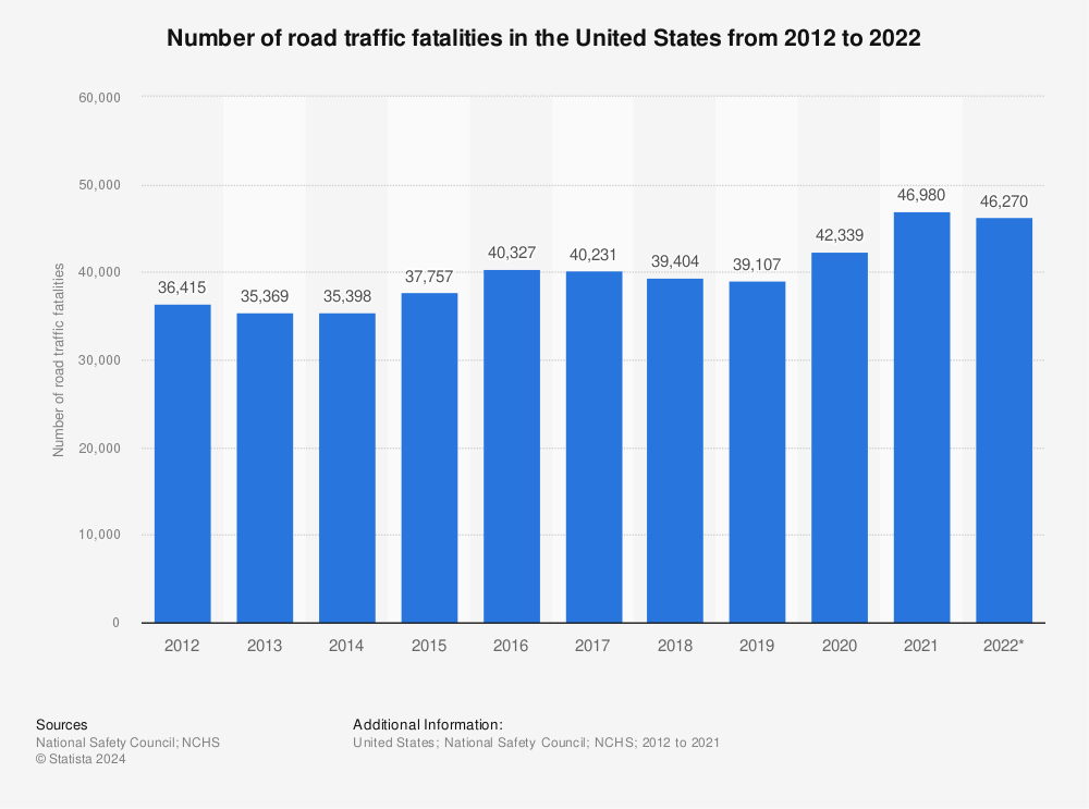
There are approximately 40,000-50,000 highway traffic fatalities each year in the US.
It is estimated that 25% of drivers on the road between 1am and 3am have been drinking.
A driver who is legally drunk is at least 13 times as likely to cause a fatal crash as a driver who has not been drinking.
We want to study government policies that can be used to discourage drunk driving.
library("AER")
data("Fatalities")
fatality.data=Fatalities
fatality.data$year <- factor(fatality.data$year)
fatality.data$mrall <- with(Fatalities, fatal/pop * 10000)
fatal.82.88.data <- subset(fatality.data, year %in% c("1982", "1988"))
Consider regressing \(FatalityRate\) (annual traffic deaths per 10,000 people in a state) on \(BeerTax\) \[\begin{alignat*}{3} \widehat{FatalityRate} = &~2.01 &{}+{} &0.15 BeerTax \qquad \text{(1982 data)} \\ &(0.15) & &(0.13) \\ \widehat{FatalityRate} = &~1.86 &{}+{} &0.44 BeerTax \qquad \text{(1988 data)} \\ &(0.11) & &(0.13) \end{alignat*}\]
9.27.1 Panel Data with Two Time Periods: “Before and After” Comparisons
Dealing with Possible OVB
The previous regression very likely suffer from OVB (which omitted variables?).
We can expand our specification to include these omitted variables, but some, like cultural attitudes towards drinking and driving in different states, would be difficult to control for.
If such omitted variables are constant across time, then we can control for them using panel data methods.
Suppose we have observations for \(T = 2\) periods for each of the \(n = 48\) states.
This approach is based on comparing the “differences’’ in the regression variables.
Modeling the Time-Constant Omitted Variable
Consider having an omitted variable \(Z_i\) that is state specific but constant across time
\[FatalityRate_{it} = \beta_0 + \beta_1 BeerTax_{it} + \beta_2 Z_i + u_{it}\]
Consider the model for the years 1982 and 1988
\[\begin{align*} FatalityRate_{i,1982} &= \beta_0 + \beta_1 BeerTax_{i,1982} + \beta_2 Z_i + u_{i,1982} \\ FatalityRate_{i,1988} &= \beta_0 + \beta_1 BeerTax_{i,1988} + \beta_2 Z_i + u_{i,1988} \end{align*}\]
Regress on Changes
Subtract the previous models for the two observed years
\[\begin{align*} FatalityRate_{i,1988}& - FatalityRate_{i,1982} = \\ &\beta_1 (BeerTax_{i,1988} - BeerTax_{i,1982}) \\ {} &+ (u_{i,1988} - u_{i,1982}) \end{align*}\]
Intuitively, by basing our regression on the change in fatalities we can ignore the time constant omitted variables.
If we regress the change in fatalities in states on the change in taxes we get \[\begin{align*} &\widehat{FatalityRate_{1988} - FatalityRate_{1982}} = \\ &\qquad {} - 0.072 - 1.04 (BeerTax_{1988} - BeerTax_{1982}) \end{align*}\]
(with standard errors \(0.064\) and \(0.26\), respectively)
We reject the hypothesis that \(\beta_1\) is zero at the 5% level.
According to this estimate an increase of $1 tax would reduce traffic fatalities by 1.04 deaths/10,000 people (a reduction by 2 of current average fatality in the data).
9.28 Fixed Effects Models
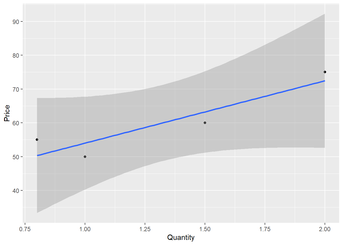
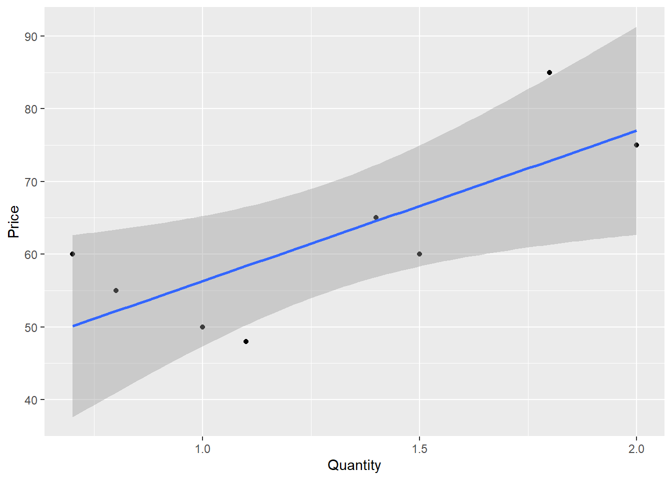
Suppose you want to learn the effect of price on the demand for back massages. You have the following data from four Midwest locations:
| Location | Year | Per capita Quantity | Price |
|---|---|---|---|
| Madison | 2003 | 0.8 | $55 |
| Peoria | 2003 | 1 | $50 |
| Milwaukee | 2003 | 1.5 | $60 |
| Chicago | 2003 | 2 | $75 |
Notice, these data are cross-sectional data for the year 2003
Quickly, eye ball the data. What is unusual about this demand function?
Graph
Panel Data You observe multiple cities for 2 years each.
| Location | Year | Per capita Quantity | Price |
|---|---|---|---|
| Madison | 2003 | 0.8 | $55 |
| Madison | 2004 | 0.7 | $60 |
| Peoria | 2003 | 1 | $50 |
| Peoria | 2004 | 1.1 | $48 |
| Milwaukee | 2003 | 1.5 | $60 |
| Milwaukee | 2004 | 1.4 | $65 |
| Chicago | 2003 | 2 | $75 |
| Chicago | 2004 | 1.8 | $85 |
Within each of the four cities, price and quantity are inversely correlated, as you would expect if demand is downward sloping.
We can see the relationship clearer if we take first differences of the data.
| Location | Year | Per capita Quantity | Price | \(\Delta\)Q | \(\Delta\)P |
|---|---|---|---|---|---|
| Madison | 2003 | 0.8 | $55 | ||
| Madison | 2004 | 0.7 | $60 | -0.1 | $5 |
| Peoria | 2003 | 1 | $50 | ||
| Peoria | 2004 | 1.1 | $48 | .1 | $2 |
| Milwaukee | 2003 | 1.5 | $60 | ||
| Milwaukee | 2004 | 1.4 | $65 | -.1 | $5 |
| Chicago | 2003 | 2 | $75 | ||
| Chicago | 2004 | 1.8 | $85 | -.2 | $10 |
A simple regression on these differences will give us our result. But what if we have more data?
More years of data
If we have lots of years of data, things get messier. We could, in principle, compute all of the differences (i.e., 2004 versus 2003, 2005 versus 2004, etc.) and then run a single regression, but there is an easier way.
Instead of thinking of each year’s observation in terms of how much it differs from the prior year for the same city, let’s think about how much each observation differs from the average for that city. With two key variables, price and quantity, we will be concerned with the following:
- Variations in prices around the mean price for each city
- Variations in quantities around the mean quantity for each city.
We want to know whether variations in the quantities (around their means) are related to variations in prices (around their means).
With our relatively small massage data set, we can do this by hand.
| Location | Year | Price | \(\bar{P}\) | Quantity | \(\bar{Q}\) |
|---|---|---|---|---|---|
| Madison | 2003 | \(\$55\) | \(\$57.5\) | 0.8 | 0.75 |
| Madison | 2004 | \(\$60\) | \(\$57.5\) | 0.7 | 0.75 |
| Peoria | 2003 | \(\$50\) | \(\$49\) | 1 | 1.05 |
| Peoria | 2004 | \(\$48\) | \(\$49\) | 1.1 | 1.05 |
| Milwaukee | 2003 | \(\$60\) | \(\$62.5\) | 1.5 | 1.45 |
| Milwaukee | 2004 | \(\$65\) | \(\$62.5\) | 1.4 | 1.45 |
| Chicago | 2003 | \(\$75\) | \(\$80\) | 2.0 | 1.9 |
| Chicago | 2004 | \(\$85\) | \(\$80\) | 1.8 | 1.9 |
| Location | Year | Price | \(\bar{P}\) | Price - \(\bar{P}\) | Quantity | \(\bar{Q}\) |
|---|---|---|---|---|---|---|
| Madison | 2003 | \(\$55\) | \(\$57.5\) | -2.5 | 0.8 | 0.75 |
| Madison | 2004 | \(\$60\) | \(\$57.5\) | 2.5 | 0.7 | 0.75 |
| Peoria | 2003 | \(\$50\) | \(\$49\) | 1 | 1 | 1.05 |
| Peoria | 2004 | \(\$48\) | \(\$49\) | -1 | 1.1 | 1.05 |
| Milwaukee | 2003 | \(\$60\) | \(\$62.5\) | -2.5 | 1.5 | 1.45 |
| Milwaukee | 2004 | \(\$65\) | \(\$62.5\) | 2.5 | 1.4 | 1.45 |
| Chicago | 2003 | \(\$75\) | \(\$80\) | -5 | 2.0 | 1.9 |
| Chicago | 2004 | \(\$85\) | \(\$80\) | 5 | 1.8 | 1.9 |
Note that by subtracting the means, we have restricted all of the action in the regression to within-city action.
Thus, we have eliminated the key source of omitted variable bias, namely, unobservable across-city differences.
Graph without adjusting for fixed effects
Graph with adjusting for fixed effects
data1 <- data1 %>% group_by(Location) %>% mutate(price_m = mean(Price), quantity_m = mean(Quantity))
data1 <- data1 %>% mutate(difprice = Price-price_m, difquantity= Quantity-quantity_m)
library(tidyverse)
data1 %>% ggplot(aes(x=difquantity, y=difprice))+geom_point()+geom_smooth(method = "lm", formula = y~x)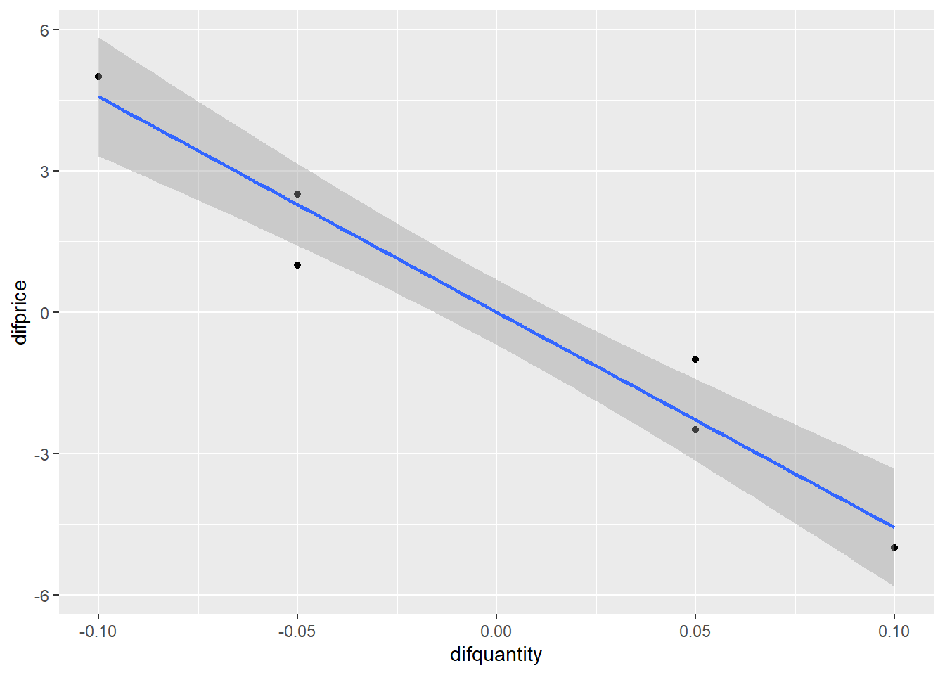
library(stargazer)
library(plm)
reg1<-lm(Price ~ Quantity, data = data1)
reg2 <-lm(difprice ~ difquantity, data = data1)
reg3 <- lm(Price ~ Quantity + factor(Location), data = data1)
reg4 <- plm(Price ~ Quantity, data = data1, model = "within", effect = "individual", index = c("Location","Year"))
stargazer::stargazer(reg1,reg2,reg3,reg4, type = "html")| Model 1 | Model 2 | Model 3 | Model 4 | |
|---|---|---|---|---|
| (Intercept) | 35.62** | 0.00 | 166.86*** | |
| (9.52) | (0.28) | (11.54) | ||
| Quantity | 20.69* | -45.71** | -45.71** | |
| (7.00) | (6.06) | (6.06) | ||
| difquantity | -45.71*** | |||
| (4.29) | ||||
| factor(Location)Madison | -75.07** | |||
| (7.06) | ||||
| factor(Location)Milwaukee | -38.07** | |||
| (2.95) | ||||
| factor(Location)Peoria | -69.86*** | |||
| (5.28) | ||||
| R2 | 0.59 | 0.95 | 1.00 | 0.95 |
| Adj. R2 | 0.53 | 0.94 | 0.99 | 0.88 |
| Num. obs. | 8 | 8 | 8 | 8 |
| ***p < 0.001; **p < 0.01; *p < 0.05 | ||||
9.29 The Fixed Effects Regression Model
We can modify our previous model
\[Y_{it} = \beta_0 + \beta_1 X_{it} + \beta_2 Z_i + u_{it}\]
as
\[Y_{it} = \beta_1 X_{it} + \alpha_i + u_{it}\]
where \(\alpha_i = \beta_0 + \beta_2Z_i\) are the \(n\) entity specific intercepts.
These are also known as entity fixed effects, since they represent the constant effect of being in entity \(i\).
Dummy Variable Fixed Effects Regression Model
Let the dummy variable \(D1_i\) be binary variable that equal 1 when \(i = 1\), 0 otherwise.
We can likewise define \(n\) dummy variables \(Dj_i\) which are equal to 1 when \(j = i\). We can write our model as
\[Y_{it} = \beta_0 + \beta_1 X_{it} + \underbrace{\gamma_2 D2_i + \gamma_3 D3_i + \cdots + \gamma_n Dn_i}_{n-1 \text{ dummy variables}} + u_{it}\]
Fixed Effects Animated
We can easily extend both forms of the fixed effects model to include multiple regressors
\[\begin{align*} Y_{it} &= \beta_1 X_{1,it} + \cdots + \beta_k X_{k,it} + \alpha_i + u_{it} \\ Y_{it} &= \beta_0 + \beta_1 X_{1,it} + \cdots + \beta_k X_{k,it}\\ {} &+ \gamma_2 D2_i + \gamma_3 D3_i + \cdots + \gamma_n Dn_i + u_{it} \end{align*}\]
9.29.1 Estimation and Inference
We now have \(k + n\) coefficients to estimate
We are not interested in estimating the entity-specific effects so we need a way to subtract them from the regression. We use an “entity-demeaned” OLS algorithm.
- We subtract the entity specific average from each variables
- We regress the demeaned dependent variable on the demeaned regressors
Taking averages of the fixed effects model \[\bar{Y}_i = \beta_1\bar{X}_i + \alpha_i + \bar{u}_i\] and subtract it from the original model \[Y_{it} - \bar{Y}_i = \beta_1(X_{it} - \bar{X}_i) + (u_{it} - \bar{u}_i)\] or \[\tilde{Y}_{it} = \beta_1 \tilde{X}_{it} + \tilde{u}_{it}\] We will discuss needed assumptions in order to carry out OLS regression and inference below.
Application to Traffic Deaths
library(plm)
regress.results.fe.only <- plm(mrall ~ beertax,
                               data=fatality.data,
                               index=c('state', 'year'),
                               effect='individual',
                               model='within')
robust.se <- vcovHC(regress.results.fe.only, method="arellano", type="HC2")
coeftest(regress.results.fe.only, vcov = robust.se)
##
## t test of coefficients:
##
## Estimate Std. Error t value Pr(>|t|)
## beertax -0.65587 0.29294 -2.2389 0.02593 *
## ---
## Signif. codes: 0 '***' 0.001 '**' 0.01 '*' 0.05 '.' 0.1 ' ' 1Time Fixed Effects
In the previous regression there is still a possibility of OVB due to effects are constant across states by different across time.
We can modify our model to
\[Y_{it} = \beta_0 + \beta_1 X_{it} + \beta_2 Z_i + \beta_3 S_t + u_{it}\]
where \(S_t\) is unobserved.
Suppose that entity specific effects (\(Z_i\)) are not present in our model but time effects are.
The same as with entity fixed effects we can model time effects as having a different intercept per time period \[Y_{it} = \beta_1 X_{it} + \lambda_t + u_{it}\] where \(\lambda_1,\dots, \lambda_T\) are the time fixed effects.
We can also use the dummy variable approach. Let \(Bs_t\) be equal to 1 if \(s = t\) and 0 otherwise.
\[Y_{it} = \beta_0 + \beta_1 X_{it} + \underbrace{\delta_2 B2_t + \cdots + \delta_T BT_t}_{T-1\text{ dummy variables}} + u_{it}\]
Application to Traffic Deaths
library(plm)
regress.results.fe.time1 <- plm(mrall ~ beertax,
                               data=fatality.data,
                               index=c('state', 'year'),
                               effect='time',
                               model='within')
robust.se <- vcovHC(regress.results.fe.time1, method="arellano", type="HC2")
coeftest(regress.results.fe.time1, vcov = robust.se)
##
## t test of coefficients:
##
## Estimate Std. Error t value Pr(>|t|)
## beertax 0.36634 0.12000 3.0527 0.002453 **
## ---
## Signif. codes: 0 '***' 0.001 '**' 0.01 '*' 0.05 '.' 0.1 ' ' 1Both Entity and Time Fixed Effects
Now to control for both \(Z_i\) and \(S_t\) we have the combined entity and time fixed effects regression model
\[Y_{it} = \beta_1 X_{it} + \alpha_i + \lambda_t + u_{it}\]
or
\[\begin{align*} Y_{it} &= \beta_0 + \beta_1 X_{it} + \gamma_2 D2_i + \cdots + \gamma_n Dn_i \\ {}&+ \delta_2 B2_t + \cdots + \delta_T BT_t + u_{it} \end{align*}\]
Application to Traffic Deaths
regress.results.fe.time <- plm(mrall ~ beertax,
                               data = fatality.data,
                               index = c('state', 'year'),
                               effect = 'twoways',
                               model = 'within')
robust.se <- vcovHC(regress.results.fe.time, method="arellano", type="HC2")
coeftest(regress.results.fe.time, vcov = robust.se)
##
## t test of coefficients:
##
## Estimate Std. Error t value Pr(>|t|)
## beertax -0.63998 0.35725 -1.7914 0.0743 .
## ---
## Signif. codes: 0 '***' 0.001 '**' 0.01 '*' 0.05 '.' 0.1 ' ' 19.30 The Fixed Effects Regression Assumptions and Standard Errors for Fixed Effects Regression
\[Y_{it} = \beta_1 X_{it} + \alpha_i + u_{it},~~i = 1, \dots,n,~~t = 1,\dots,T.\]
- FE.A.1: \(u_{it}\) has conditional mean zero: \(E[u_{it}|X_{i1}, \dots, X_{iT}, \alpha_i] = 0\).
- FE.A.2: \((X_{i1}, \dots, X_{iT}, u_{i1},\dots,u_{iT})\), \(i = 1,\dots,n\) are i.i.d. draws from their joint distribution.
- FE.A.3: Large outliers are unlikely.
- FE.A.4: No perfect multicollinearity.
Serial Correlation of Standard Errors
An important assumption for fixed effects regressions is FE.A.2
The assumption requires variables to be independent across entities but not necessarily within entities.
For example any \(X_{it}\) and \(X_{is}\) for \(t \ne s\) can be correlated: this is called autocorrelation or serial correlation.
Autocorrelation is common in time series and panel data:
what happens in one period is probably correlated with what happens in other periods for the same entity.
The same can be said for the error terms \(u_{it}\).
For that reason we need to use heteroskedasticity- and autocorrelation-consistent (HAC) standard errors.
Let us test for Serial Correlation in R
##
##  Breusch-Godfrey/Wooldridge test for serial correlation in panel models
##
## data:  mrall ~ beertax
## chisq = 54.188, df = 7, p-value = 2.159e-09
## alternative hypothesis: serial correlation in idiosyncratic errors
Robust Standard Errors
We will use two types of robust standard erros to deal with the problem of heteroskedasticity.
- General Robust Standard errors
- Clustered Robust Standard Errors
Robust Standard Errors
In regression and time-series modelling, basic forms of models make use of the assumption that the errors or disturbances \(u_i\) have the same variance across all observation points.
When this is not the case, the errors are said to be heteroscedastic, or to have heteroscedasticity, and this behaviour will be reflected in the residuals \(u_i\) estimated from a fitted model.
Heteroscedasticity-consistent standard errors are used to allow the fitting of a model that does contain heteroscedastic residuals.
The first such approach was proposed by Huber (1967), and further improved procedures have been produced since for cross-sectional data, time-series data and GARCH estimation.
How to test for heteroscedasticity in R
We use the Breusch-Pagan test to detect heteroskedasticity. The null hypothesis is homoscedasticity in the errors.
library(lmtest)
bptest(mrall ~ beertax+factor(state)+factor(year), data = fatality.data, studentize=F)
##
## Breusch-Pagan test
##
## data: mrall ~ beertax + factor(state) + factor(year)
## BP = 295.57, df = 54, p-value < 2.2e-16Clustered Robust Standard Errors
Let’s say that you want to relax the Gauss-Markov homoscedasticity assumption, and account for the fact that there may be several different covariance structures within your data sample that vary by a certain characteristic - a “cluster” - but are homoscedastic within each cluster.
For example, say you have a panel data set with a bunch of different test scores from different schools around the country.
You may want to cluster your sample by state, by school district, or even by town.
Economic theory and intuition will guide you in this decision.