Chapter 11 Difference in Differences | Econometrics for Business Analytics

11.1 Framework

Recall the potential outcome framework. When we estimate a treatment-control contrast what we get is: \[E(Y|D=1)-E(Y|D=0)=\delta+E(Y_0|D=1)-E(Y_0|D=0)\] Where \(\delta\) is the ATE.

This equation says that the average of the treated group minus the average of the control group is the average treatment effect plus selection bias (AKA omitted variable bias in the regression framework).

11.1.1 Parallel Trends

We will now explore another way to get rid of the selection bias (i.e. \(E(Y_0|D=1)-E(Y_0|D=0)\))

Suppose we have data on the outcome variable for our treatment and control group from a previous period. Call this \(Y_{pre}\).

Now suppose further that: \[E(Y_0|D=1)-E(Y_{pre}|D=1)=E(Y_0|D=0)-E(Y_{pre}|D=0)\] This equation says the change in the treatment group is equal to the change in the control group when neither group receives the active treatment.

This assumption is known as the parallel trends assumptions and is crucial for getting compelling estimates in the dif-in-dif framework.

It says that if the treatment group had never been treated, the average change in the outcome variable would have been identical to the average change in the outcome variable for the control group.

How plausible this assumption is depends upon the given study you are examining.

For now, let’s assume it is true, and see how this can help us kill the selection bias.

11.1.2 Our first Causal Model:DiD

Difference in Differences (DiD): exploits natural experiments in observational data to obtain causal estimates.

Need items

Random (or quasi random) assignment of treatment and control groups.
A pre-period and a post-period for both groups.
No sample selection bias.
Must have parallel trends.

11.1.3 DAG

Causal Pathway Illustration: Z (confounder) is the cause of both X (independent variable) and Y (dependent variable) and thus, obscures the relationship between X and Y.

Figure 11.1: Causal Pathway Illustration: Z (confounder) is the cause of both X (independent variable) and Y (dependent variable) and thus, obscures the relationship between X and Y.

11.1.4 DiD

The DiD estimator is a version of the Fixed Effects Model can be used with both

repeated cross-sectional (easier to obtain)
and panel data. (harder to obtain)

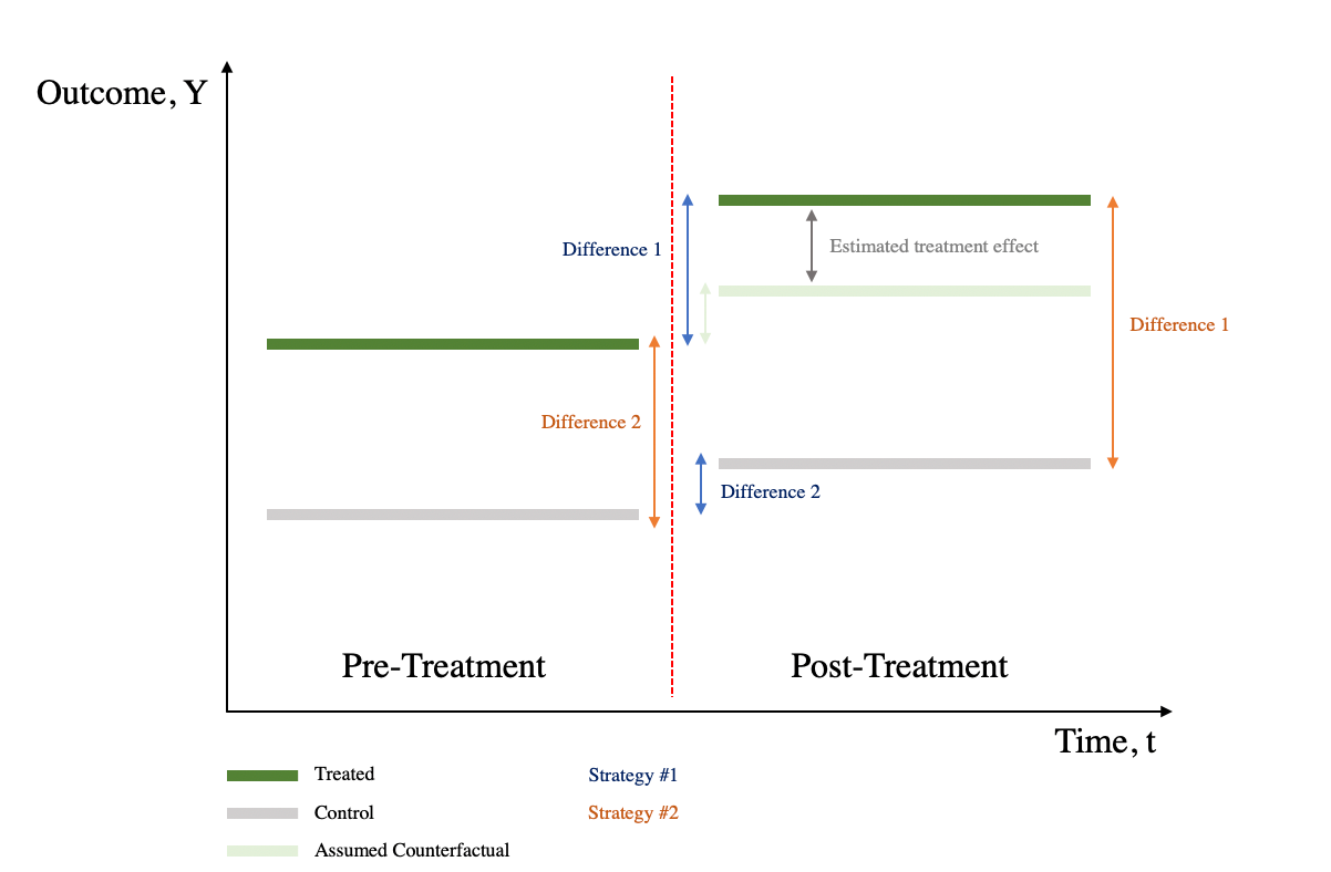
DiD is a combination of time-series difference (compares outcomes across pre-treatment and post-treatment periods) and cross-sectional difference (compares outcomes between treatment and control groups).

11.1.5 Intuition

There are two equivalent strategies to think about the two “differences”:

11.1.6 Visually DID

Visually, the DiD is the difference between these two changes:

changes in outcomes from pre-treatment to post-treatment
changes in outcomes between treatment and control groups

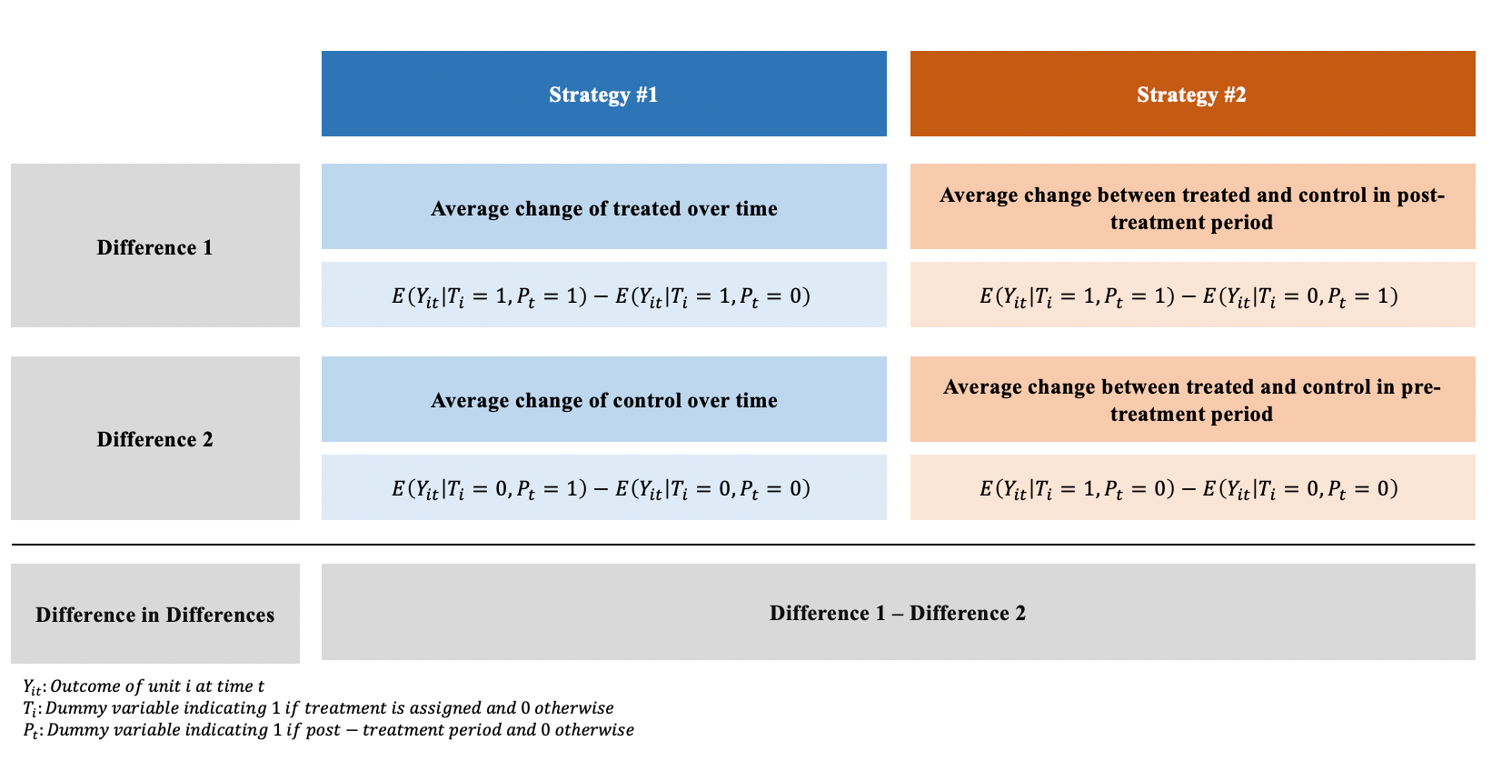
11.2 Regression DiD

\[y_{it}=\beta_0+\beta_1 Post_i+\beta_2 Treat_t+\beta_3 Treat_i*Post_t+\gamma X_{it}+e_{it}\] While it is possible to obtain the DiD estimator by calculating the means by hand, using a regression framework may be more advantageous as it:

outputs standard errors for hypothesis testing
can be easily extended to include multiple periods and groups
allows the addition of covariates

11.2.1 Treatment Effect

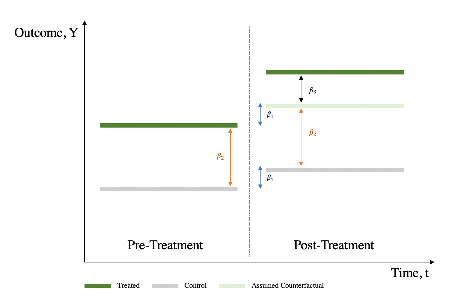
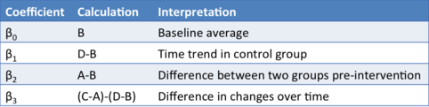
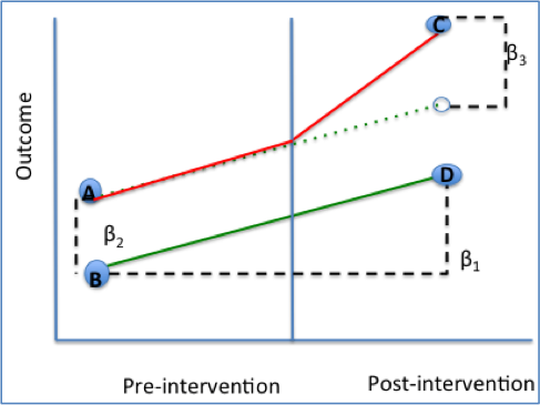
11.2.2 Interpreting the Coefficients

\(\beta_0\): Average value of y in the control group during the preperiod.
\(\beta_1\): Average change in y from the first to the second time period that is common to both groups
\(\beta_2\): Average difference in y between the two groups that is common in both time periods
\(\beta_3\): Average differential change in y from the first to the second time period of the treatment group relative to the control group

11.2.3 The coefficients visually

11.2.4 Difference in Differences: Animated

11.2.5 Difference in Differences: Differences in Means Example

11.2.6 Difference in Differences: Graphical Approach

\[\begin{align*}Y&= \beta_0 + \beta_1*[Time] + \beta_2*[Intervention] \\ &+ \beta_3*[Time*Intervention] + \beta_4*[Covariates]+\epsilon\end{align*}\]

11.3 Parallel Trend Assumption

The parallel trend assumption is the most critical of the above the four assumptions to ensure internal validity of DID models and is the hardest to fulfill.

It requires that in the absence of treatment, the difference between the ‘treatment’ and ‘control’ group is constant over time.

Although there is no statistical test for this assumption, visual inspection is useful when you have observations over many time points.

It has also been proposed that the smaller the time period tested, the more likely the assumption is to hold.

Violation of parallel trend assumption will lead to biased estimation of the causal effect.

11.3.1 Parralel Trend Assumption: Met

11.3.2 Parralel Trend Assumption: Violated

11.4 Generalized DiD

We can generalize the DiD model for multiple time periods. - Very useful for policy adoption as they tend to happened at different times

\[y_{it}=\beta_0+\alpha_i+\delta_t+\beta_3 d_{it}+\gamma X_{it}+e_{it}\]

\(\alpha_i\): Individual fixed effects that change across individuals (state-specific characteristics, individual’s gender, etc.)
\(\delta_t\): Time fixed effects that change across time (e.g. year dummies to allow intercept to vary across different years)
\(d_{it}\): dummy variable which equals 1 if the unit of observation is in the post-treatment period (in contrast to Pt equals 1 in the second time period)

11.5 Threats to Validity

Parallel Trends Assumption is violated

Try a placebo treatment
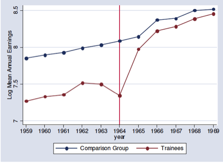
Visually inspect pre-trends using an event study

Difference in composition

Covariates can mitigate this problem
The people you are examining should not change too much within their group.

Extrapolation

Depending on the setting of interest, results may be unable to generalise to other populations or even a longer time frame.

11.6 Silly Example

Consider a chili cheese hot dog 1. What is the cheese effect? 2. What is the chili effect? 3. What is the chili * cheese effect?

11.6.1 A simple example in R

library(foreign)
mydata = read.dta("http://dss.princeton.edu/training/Panel101.dta")
mydata$y <- mydata$y/1000000000
# First, let's create a post time variable
mydata$time = ifelse(mydata$year >= 1994, 1, 0)
# Second, let's create a treated group
mydata$treated = ifelse(mydata$country == "E" |
mydata$country == "F" |
mydata$country == "G", 1, 0)
# Third, the interaction term
mydata$did = mydata$time * mydata$treated

11.6.2 4 ways to do DiD

I will show you a couple of different ways to run DiD in R.

library(plm) #panel linear model
library(lfe) #linear fixed effect model
library(fixest)
reg1<-lm(y~time+treated+did, data=mydata)
reg2<-lm(y~time*treated, data=mydata)
reg3<-plm(y~did, data = mydata, index = c("country","year"), effect = "twoways", model = "within") 
reg4 <-felm(y~did | country + year, data = mydata)
reg5 <-feols(y~did | country + year, data = mydata)

	(1)	(2)	(3)	(4)	(5)
(Intercept)	0.358	0.358
	(0.738)	(0.738)
time	2.289	2.289
	(0.953)	(0.953)
treated	1.776	1.776
	(1.128)	(1.128)
did	-2.520		-2.520	-2.520	-2.520
	(1.456)		(1.328)	(1.328)	(1.086)
time × treated		-2.520
		(1.456)
Num.Obs.	70	70	70	70	70
R2	0.083	0.083	0.064	0.387	0.387
R2 Adj.	0.041	0.041	-0.219	0.202	0.202
R2 Within					0.064
R2 Within Adj.					0.046
AIC	356.1	356.1	321.9	353.9	351.9
BIC	367.4	367.4	326.4	394.3	390.1
Log.Lik.	-173.055	-173.055
F	1.984	1.984
RMSE	2.87	2.87	2.34	2.34	2.34
Std.Errors					by: country
FE: country					X
FE: year					X

11.7 Event Study

library(ggplot2)
reg6 <- feols(y~ i(year,treated,1994)|country + year, data = mydata)
coefplot(reg6)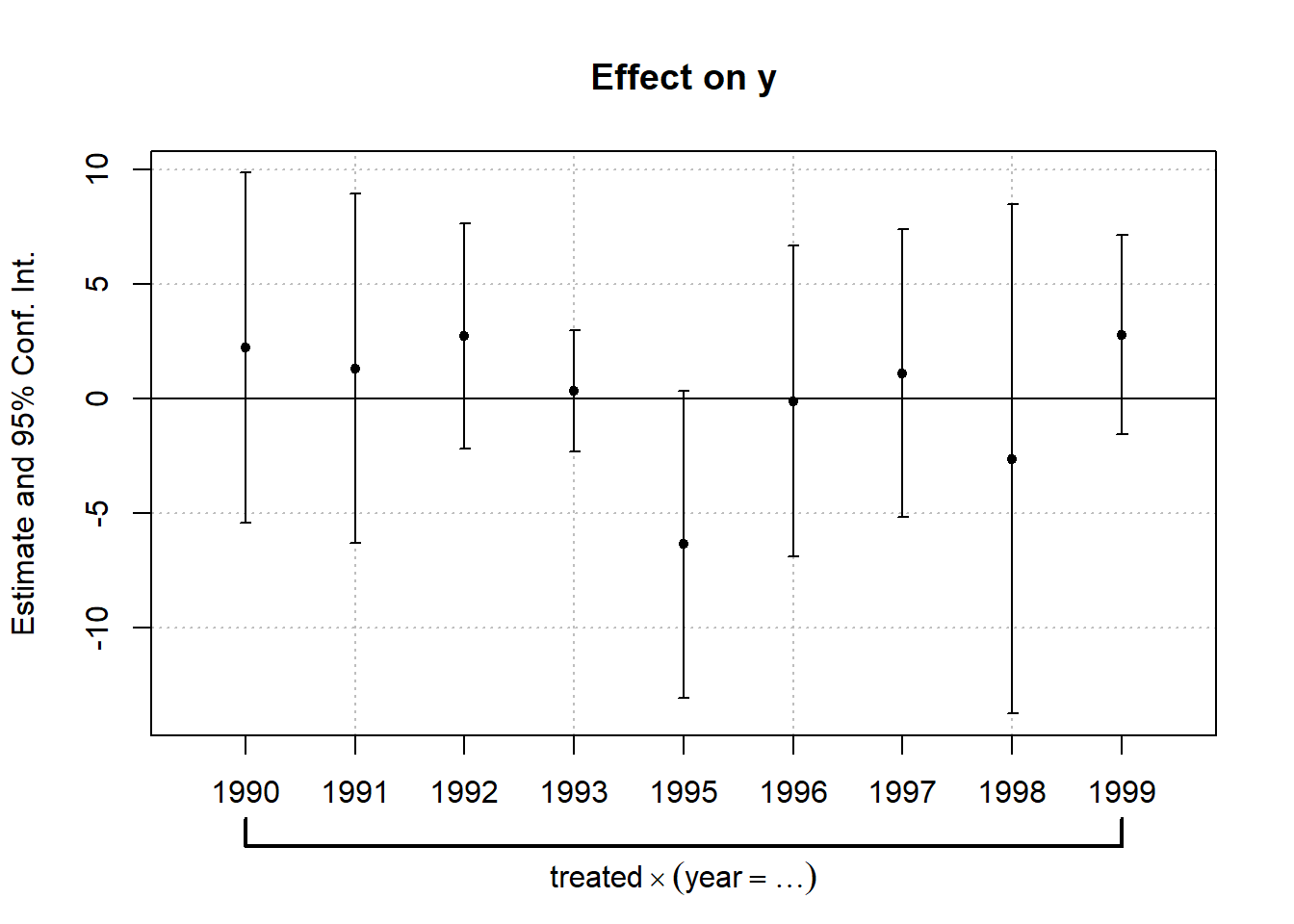

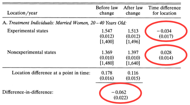
11.8 Dif-in-Dif in Practice

Case study: who pays for mandated childbirth coverage?

When the government mandates employers to provide benefits, who is really footing the bill?

Is it the employer?
Or is it the employee who pays for it indirectly in the form of a pay cut?

This analysis is first conducted by Jonathan Gruber in 1994, an MIT Professor who serves as the director of the Health Care Program at the National Bureau of Economic Research (NBER). To date, The Incidence of Mandated Benefits remains one of the most influential paper in healthcare economics.

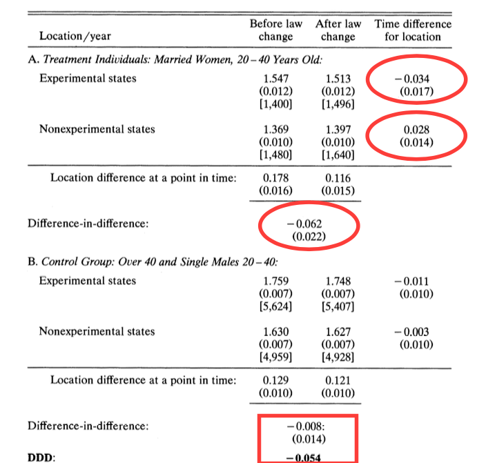
11.8.1 Timeline

Understanding the timeline is important for identifying the causal effect:

Before 1978: there was limited health care coverage for childbirth.

1975-1979: a subset of states passed laws, mandating the health care coverage of childbirth.

Starting in 1978: federal legislation mandates the health care coverage of childbirth for all states.

11.8.2 Difference-in-Differences Table

11.8.3 The Legendary Triple Dif

11.8.4 Dif-in-Dif in R - Manual Calculation

require(foreign)
eitc<-read.dta("https://github.com/CausalReinforcer/Stata/raw/master/eitc.dta")
# Create two additional dummy variables to indicate before/after
# and treatment/control groups.

# the EITC went into effect in the year 1994
eitc$post93 = as.numeric(eitc$year >= 1994)

# The EITC only affects women with at least one child, so the
# treatment group will be all women with children.
eitc$anykids = as.numeric(eitc$children >= 1)

# Compute the four data points needed in the DID calculation:
a = sapply(subset(eitc, post93 == 0 & anykids == 0, select=work), mean)
b = sapply(subset(eitc, post93 == 0 & anykids == 1, select=work), mean)
c = sapply(subset(eitc, post93 == 1 & anykids == 0, select=work), mean)
d = sapply(subset(eitc, post93 == 1 & anykids == 1, select=work), mean)

# Compute the effect of the EITC on the employment of women with children:
(d-c)-(b-a)

##       work 
## 0.04687313

11.8.5 Dif-in-Dif in R - Regression

\[work=\beta_0+\delta_0posst93+\beta_1anykids+\delta_1(anykids*post93)+\epsilon\]

reg1 = lm(work ~ post93 + anykids + post93*anykids, data = eitc)
summary(reg1)

## 
## Call:
## lm(formula = work ~ post93 + anykids + post93 * anykids, data = eitc)
## 
## Residuals:
##     Min      1Q  Median      3Q     Max 
## -0.5755 -0.4908  0.4245  0.5092  0.5540 
## 
## Coefficients:
##                 Estimate Std. Error t value Pr(>|t|)    
## (Intercept)     0.575460   0.008845  65.060  < 2e-16 ***
## post93         -0.002074   0.012931  -0.160  0.87261    
## anykids        -0.129498   0.011676 -11.091  < 2e-16 ***
## post93:anykids  0.046873   0.017158   2.732  0.00631 ** 
## ---
## Signif. codes:  0 '***' 0.001 '**' 0.01 '*' 0.05 '.' 0.1 ' ' 1
## 
## Residual standard error: 0.4967 on 13742 degrees of freedom
## Multiple R-squared:  0.0126, Adjusted R-squared:  0.01238 
## F-statistic: 58.45 on 3 and 13742 DF,  p-value: < 2.2e-16

11.8.6 Create Plot

# Take average value of 'work' by year, conditional on anykids
minfo = aggregate(eitc$work, list(eitc$year,eitc$anykids == 1), mean)
# rename column headings (variables)
names(minfo) = c("YR","Treatment","LFPR")

# Attach a new column with labels
minfo$Group[1:6] = "Single women, no children"
minfo$Group[7:12] = "Single women, children"
#minfo

require(ggplot2)    #package for creating nice plots

qplot(YR, LFPR, data=minfo, geom=c("point","line"), colour=Group,
xlab="Year", ylab="Labor Force Participation Rate")+geom_vline(xintercept = 1994)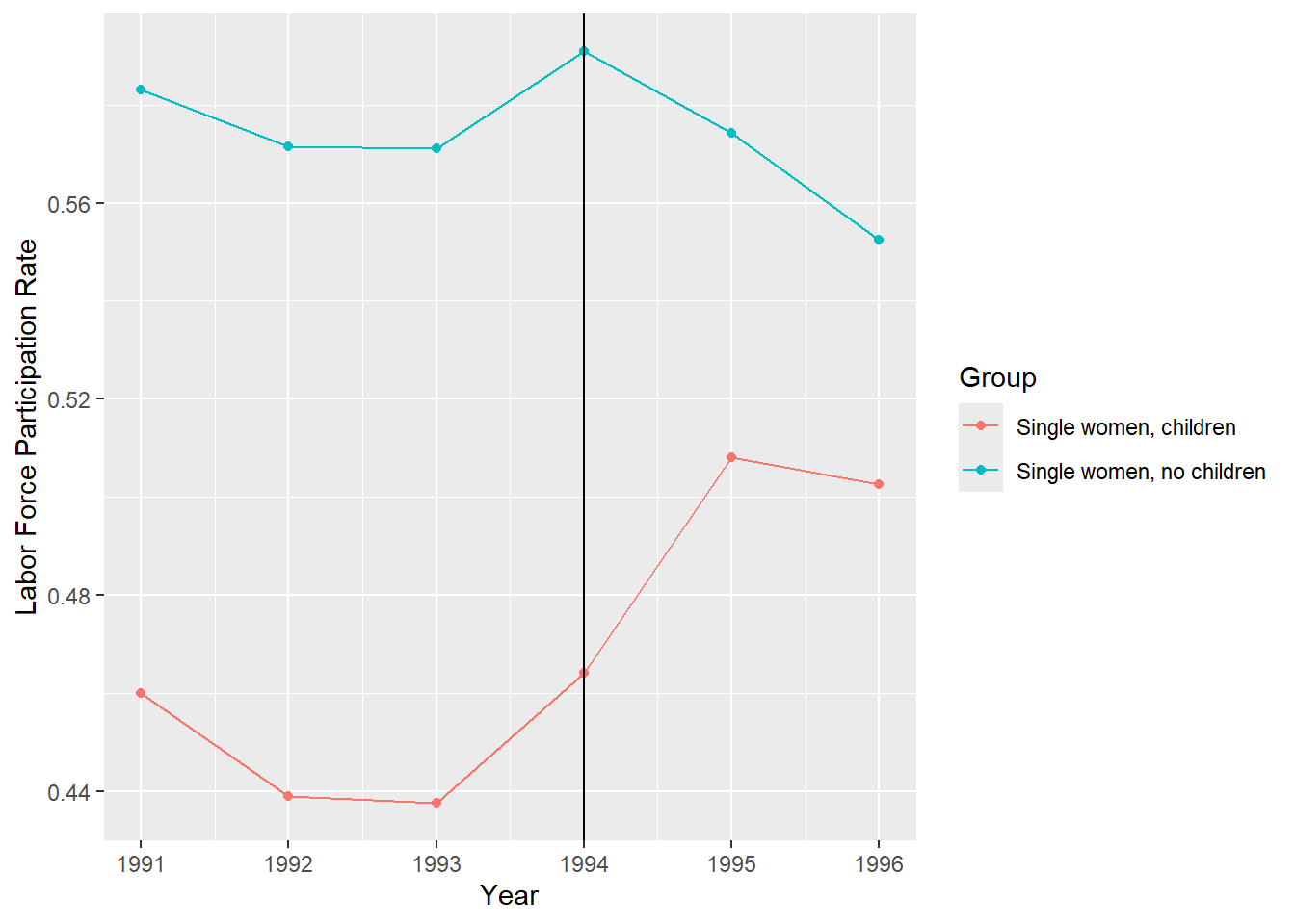

11.9 Strengths and Limitations

11.9.1 Strengths

Intuitive interpretation
Can obtain causal effect using observational data if assumptions are met
Can use either individual and group level data
Comparison groups can start at different levels of the outcome. (DID focuses on change rather than absolute levels)
Accounts for change/change due to factors other than intervention

11.9.2 Limitations

Requires baseline data & a non-intervention group
Cannot use if intervention allocation determined by baseline outcome
Cannot use if comparison groups have different outcome trend (Abadie 2005 has proposed solution)
Cannot use if composition of groups pre/post change are not stable

11.9.3 BEST PRACTICES

Be sure outcome trends did not influence allocation of the treatment/intervention
Acquire more data points before and after to test parallel trend assumption
Use linear probability model to help with interpretability
Be sure to examine composition of population in treatment/intervention and control groups before and after intervention
Use robust standard errors to account for autocorrelation between pre/post in same individual
Perform sub-analysis to see if intervention had similar/different effect on components of the outcome

11.10 New Developments

The basic difference in difference model we have discussed assume a constant treatment effect regardless across groups. The two way fixed effects (TWFE) approach we have used has come under scrutiny.

When treatment adoption is staggered (i.e. not everyone in the treatment group receive the treatment at the same time) and/or the effects are heterogenous (some people respond to the treatment more than others) plus the effect is not constant overtime, then there could be a bias introduced by the TWFE approach to dif-in-dif.

The bias is caused by how TWFE estimates the treatment effect. It takes a weighted average of the comparison groups. Let’s assume there are three different groups: control (i.e. never treated), early treated, and late treated.

The good comparisons that TWFE does is compare the control to the early treated and the control to the late treated separately. However, TWFE effects also compares the early treated to the late treated. This is known as the forbidden comparison. In this case, the early treated units may “act” as a control group for the later treated units. But this shouldn’t make sense because, they are already treated!!

There are many solutions now proposed to this problem but they are beyond the scope of this class. The current best summary of the problem and solutions can be found at this (link)[https://asjadnaqvi.github.io/DiD/]