Week 9 Transforming
The raw scores (observed score) of a test can be hard to interpret. For example, a score of 16 from a test does not tell how well an examinee did on that test. Another limitation of raw scores is that two test scores from two different tests are difficult to compare. For these matters, transformation of raw scores can aid in the interpretation of test scores. In this chapter, students will learn three types of raw-score transformations.
Percentiles
Standardized Scores
Normalized Scores
The three transformation methods discussed in this chapter are monotonic transformations, that is, the rank of the scores in a sample will not be altered after the transformation.
Let’s assume that test1 is designed to measure the math ability of students. This data set contains responses from 100 examinees on 20 items.
## [1] 100 209.1 Percentiles
Percentiles represent the percent of people at or below a trait value in the norm group. The frequency distributions of raw scores can be used to estimate percentiles associated with the trait value given the two assumptions:
Each raw score represents a range of trait values.
Every trait value in the range is equally likely to occur (i.e., an uniform distribution)
9.1.1 Frequency Distribution
The table() function returns the frequency table.
You can obtain the cumulative frequency by using cumsum() function.
##   4   5   6   7   8   9  10
##   3   4   5   7  11  17  32
##  11  12  13  14  15  16  17
##  42  56  67  74  84  93  95
##  18  19
##  98 100
The below code creates a frequency table.
The object freq_table has three columns. The first column shows the scores, the second shows the frequency of each score, and the third column represents the cumulative frequency of each score. Let’s change the column names as “Scores”, “Freq” and “CumFreq”.
##    Scores Freq CumFreq
## 4       4    3       3
## 5       5    1       4
## 6       6    1       5
## 7       7    2       7
## 8       8    4      11
## 9       9    6      17
## 10     10   15      32
## 11     11   10      42
## 12     12   14      56
## 13     13   11      67
## 14     14    7      74
## 15     15   10      84
## 16     16    9      93
## 17     17    2      95
## 18     18    3      98
## 19     19    2     100
9.1.2 Calculating Percentile
A raw score of 10 represents trait score, or math ability score, [9.5, 10.5]. And we assume that every trait value in the range is equally likely to occur. Therefore, for score 10, all trait values between 9.5 and 10.5 are equally likely to occur. We can estimate the number of examinees with math ability at or below 10 by \(32 - \frac{15}{2} = 24.5\). Or from the freq_table,
## [1] 24.5Using a for loop, let’s calculate the percentiles corresponding to scores from 4 to 19. 4 and 19 are the minimum and the maximum values of the raw scores.
scores <- min(X):max(X)
percentiles <- numeric(length(scores)) # output vector
for (i in 1:length(scores)) {
  score <- scores[i]
  num_below <- freq_table[which(freq_table[, 1] == score), 3] - freq_table[which(freq_table[, 1] == score), 2] / 2
  percentiles[i] <- num_below / length(X) * 100
}
percentiles
## [1] 1.5 3.5 4.5 6.0 9.0
## [6] 14.0 24.5 37.0 49.0 61.5
## [11] 70.5 79.0 88.5 94.0 96.5
## [16] 99.0## scores percentiles
## [1,] 4 1.5
## [2,] 5 3.5
## [3,] 6 4.5
## [4,] 7 6.0
## [5,] 8 9.0
## [6,] 9 14.0
## [7,] 10 24.5
## [8,] 11 37.0
## [9,] 12 49.0
## [10,] 13 61.5
## [11,] 14 70.5
## [12,] 15 79.0
## [13,] 16 88.5
## [14,] 17 94.0
## [15,] 18 96.5
## [16,] 19 99.09.1.3 Trait Value Corresponding to Given Percentile
We can find the trait value falling at certain percentile. For example, what is the trait value falling at 15% percentile? From the freq_table we can tell that the 15% percentile should be somewhere between 8 and 9. Below formula illustrates the calculation of a trait value corresponding to the 15% percentile.

\[8.5 + \frac{15-11}{17-11} (9.5-8.5) = 8.5 + \frac{4}{6}(1) \approx 9.17 \]
The below function percentile_score takes a matrix freq_table and a scalar percentile as inputs, and returns the trait value corresponding to the input percentile.
percentile_score <- function(freq_table, percentile){
n <- sum(freq_table[, 2]) # number of samples
num <- percentile * n
u <- which(freq_table[, 3] >= num)[1]
l <- which(freq_table[, 3] <= num)[sum(freq_table[,3] <= num)]
if(u == l){
trait_val <- freq_table[l, 1] + 0.5
}else{
trait_val <- freq_table[l, 1] + 0.5 + (num - freq_table[l, 3]) / (freq_table[u, 3] - freq_table[l, 3])
}
trait_val
}
percentile_score(freq_table, .15)## [1] 9.166667## [1] 17.59.2 Standard and Standardized Scores
The standard scores, often called Z scores, can be obtained as:
\[Z = \frac{X - \mu_X}{\sigma_X}\]
## [1] 2.620126e-16## [1] 1If the raw score distribution is approximately normal, we can easily find the percentile of an examinee’s test score using the pnorm() function. Below code will print the percentile of the first five examinees’ test scores.
## [1] 0.2567862 0.8125903
## [3] 0.2567862 0.1021149
## [5] 0.3649976One disadvantage of using standard scores is that about half of the scores are negative because the mean is always zero. Most people prefer not to deal with negative numbers as test scores, and therefore use the standardized scores. Standardized scores are obtained from the raw scores (or the standard scores) by linear transformations.
\[Y = \sigma^*Z + \mu^*\]
If we set \(\sigma^* = 10, \mu^* = 50\), we can obtain the standardized score \(Y\) with mean 50 and standard deviation 10.
## [1] 50## [1] 10Again, we can calculate the percentile of the examinee’s test score using pnorm() function, but this time we have to use the normal distribution with mean of 50 and standard deviation of 10.
## [1] 0.2567862 0.8125903
## [3] 0.2567862 0.1021149
## [5] 0.36499769.3 Normalized Scores
If the standardized scores are not normally distributed, it is difficult to compare scores on two standardized scales. In this case we can force the transformed scores to have a normal distribution. Normalization is appropriate when the underlying trait is assumed to be normally distributed. Normalization usually involves three steps:
Step 1: Transform the raw scores to percentiles.
Step 2: Find the z-score in the standard normal distribution corresponding to each percentile.
Step 3 (Optional): Transform theses z-scores to scaled scores with a desired mean and standard deviation.
Two commonly used normalized scores are the T-scores and the stanines.
9.3.1 T-scores
T-scores are normalized scores with \(\mu= 50\) and \(\sigma = 10\). To obtain T-scores, we first need to transform the raw scores to percentiles for all examinees.
##       scores percentiles
##  [1,]      4         1.5
##  [2,]      5         3.5
##  [3,]      6         4.5
##  [4,]      7         6.0
##  [5,]      8         9.0
##  [6,]      9        14.0
##  [7,]     10        24.5
##  [8,]     11        37.0
##  [9,]     12        49.0
## [10,]     13        61.5
## [11,]     14        70.5
## [12,]     15        79.0
## [13,]     16        88.5
## [14,]     17        94.0
## [15,]     18        96.5
## [16,] 19 99.0p <- numeric(length(X))
for (i in 1:length(X)) {
p[i] <- percentiles[which(X[i] == scores)]
}
z_score <- qnorm(p / 100)
T_score <- z_score * 10 + 50Or loop over the scores which could be faster.
9.3.2 Stanines
Stanines are one-digit normalized scores with mean of 5 and standard deviation of approximately 2. Transformations to stanines can be done by following the below table.
| PERCENTILE_RANGE | STANINE |
|---|---|
| 96 - 100 | 9 |
| 89 - 96 | 8 |
| 77 - 89 | 7 |
| 60 - 77 | 6 |
| 40 - 60 | 5 |
| 23 - 40 | 4 |
| 11 - 23 | 3 |
| 4 - 11 | 2 |
| 0 - 4 | 1 |
Below function will return a stanine score corresponding to a specific percentile score.
my_stanine <- function(percent) {
  ranges <- c(0, 4, 11, 23, 40, 60, 77, 89, 96, 100)
  stanine <- NA
  for(i in 1:9){
    if(percent > ranges[i] && percent <= ranges[i + 1]) {
      stanine <- i
    }
  }

  stanine
}
For example, the stanine score corresponding to percentile score 30 is 4.
## [1] 4Now we can obtain the stanine for all examinees using a for loop.
##   [1] 4 7 4 2 4 4 7 4 4 4 6 3
##  [13] 5 5 7 2 7 8 1 5 5 4 6 9
##  [25] 9 4 7 4 4 5 5 5 4 6 4 6
##  [37] 8 4 4 6 6 7 5 5 6 9 6 1
##  [49] 4 4 3 2 4 7 2 6 6 4 7 3
##  [61] 6 7 3 6 7 9 2 3 5 7 5 6
##  [73] 2 1 4 4 6 7 7 4 5 5 2 7
##  [85] 6 9 7 4 5 1 7 7 7 6 6 3
## [97] 4 4 6 7## [1] 5.08## [1] 1.92632When reporting the test result, we can show the raw scores along with percentiles, T-scores, and stanines for all examinees.
result <- cbind(X, p, T_score, stanine)
colnames(result) <- c("Raw_Score", "Percentile", "T_Score", "Stanine")
head(result, 10)
## Raw_Score Percentile
## [1,] 10 24.5
## [2,] 15 79.0
## [3,] 10 24.5
## [4,] 8 9.0
## [5,] 11 37.0
## [6,] 11 37.0
## [7,] 15 79.0
## [8,] 10 24.5
## [9,] 11 37.0
## [10,] 10 24.5
## T_Score Stanine
## [1,] 43.09691 4
## [2,] 58.06421 7
## [3,] 43.09691 4
## [4,] 36.59245 2
## [5,] 46.68147 4
## [6,] 46.68147 4
## [7,] 58.06421 7
## [8,] 43.09691 4
## [9,] 46.68147 4
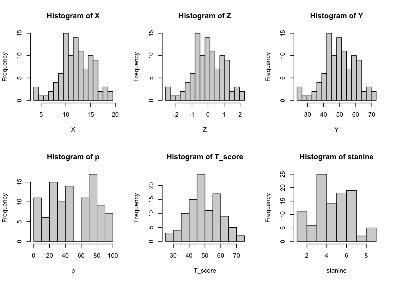
## [10,] 43.09691 4Below figure shows the histograms of the six scores: Raw score (X), Standard score (Z), Standardized score (Y), Percentile score (p), T-score (T_score), and Stanine (stanine).
br <- seq(3.5, 19.5, 1)

par(mfrow=c(2, 3))
hist(X, breaks = br)
hist(Z, breaks = (br - mean(X)) / sd(X))
hist(Y, breaks = (br - mean(X)) / sd(X) * 10 + 50)
hist(p)
hist(T_score)
hist(stanine)