Week 8 Test Construction
Suppose that we developed a new test containing \(N\) newly written items. The test is designed to measure a unidimensional latent construct. Also, the test items are assumed to be essentially \(tau-\)equivalent. This \(N\)-item test is administered to a pretest sample. Based on the pretest data, we want to choose \(k \leq N\) items, to be included on the operational test. In other words, the remaining \(N-k\) items will not be used on the actual test. The test is used to predict a criterion variable/score \(Y\). In the pretest, we collected examinees’ criterion scores, \(Y\)s, as well.
In this chapter, we will revisit the CTT item analysis. And then we will discuss how we can use these items related statistics to decide which \(k\) items to include in our test.
8.1 Item Analysis: Item Reliability and Validity Indices
Here, we are going to use the two data sets.
responses: A \(1000 \times 40\)data.framecontaining the pretest responses to \(40\) items from \(1,000\) examinees.Y: A vector length of \(1,000\) containing the examinees’ criterion scores.
responses <- read.table("https://raw.githubusercontent.com/sunbeomk/PSYC490/main/responses.txt")
Y <- read.table("https://raw.githubusercontent.com/sunbeomk/PSYC490/main/criterion.txt")
Let’s check the responses from the first 6 examinees.
Next is the criterion scores from the first 6 examinees.
For each item \(i\), we are going to obtain:
Item difficulty
Item discrimination
Item-score SD
And using the three item statistics above, we can obtain:
Item reliability
Item validity
Note: The item reliability and the item validity are different from the reliability and the validity of a test. In this chapter, we are focusing on the item-level statistics.
8.1.1 Item Difficulty
The item difficulty is proportion of examinees who responded correctly on the item, i.e., \[p_i = \frac{\sum_{p=1}^n X_{pi}}{n}\].
##    V1    V2    V3    V4    V5
## 0.630 0.384 0.705 0.577 0.685
##    V6    V7    V8    V9   V10
## 0.425 0.439 0.359 0.328 0.560
##   V11   V12   V13   V14   V15
## 0.676 0.602 0.516 0.489 0.778
##   V16   V17   V18   V19   V20
## 0.606 0.531 0.324 0.493 0.325
##   V21   V22   V23   V24   V25
## 0.520 0.627 0.243 0.388 0.510
##   V26   V27   V28   V29   V30
## 0.247 0.389 0.621 0.428 0.340
##   V31   V32   V33   V34   V35
## 0.339 0.400 0.443 0.279 0.457
##   V36   V37   V38   V39   V40
## 0.199 0.445 0.281 0.171 0.194
8.1.2 Item Discrimination
This is the point-biserial correlation between item score (0/1) and total score (\(X\)), given by \[r_{iX}=r_{pbis} = \left[\frac{\bar X_1 - \bar X_0}{S_X}\right]\sqrt{\frac{n_1 n_0}{n(n-1)}},\] or, more simply, the Pearson correlation between dichotomous item score and total score.
In previous chapters, we learned how to compute this:
total <- rowSums(responses) # total score

discrimination <- numeric(ncol(responses))  # outcome vector
for (i in 1:ncol(responses)) {
  discrimination[i] <- cor(responses[, i], total) # Pearson correlation between the i-th item score and the total score
}
discrimination
## [1] 0.2003023 0.2633101
## [3] 0.2157009 0.2513577
## [5] 0.3098860 0.2639948
## [7] 0.2631635 0.3384545
## [9] 0.3131245 0.3318597
## [11] 0.2618446 0.3135515
## [13] 0.3345164 0.3089618
## [15] 0.3208180 0.3625530
## [17] 0.3684249 0.3470304
## [19] 0.3606028 0.3569275
## [21] 0.3955714 0.3782499
## [23] 0.3770550 0.3779781
## [25] 0.4531812 0.3824007
## [27] 0.4378612 0.4120439
## [29] 0.4788896 0.4611929
## [31] 0.3954019 0.4476655
## [33] 0.4963732 0.4260595
## [35] 0.4204738 0.3638530
## [37] 0.4955949 0.4764930
## [39] 0.4339662 0.49747438.1.3 Item-score SD
This is the standard deviation (SD) of the observed score (0/1) on an item. We know that this is equal to \[s_i = \sqrt{p_i(1-p_i)}.\]
To compute this in r:
##        V1        V2        V3
## 0.4828043 0.4863579 0.4560428
##        V4        V5        V6
## 0.4940354 0.4645159 0.4943430
##        V7        V8        V9
## 0.4962651 0.4797072 0.4694848
##       V10       V11       V12
## 0.4963869 0.4680000 0.4894854
##       V13       V14       V15
## 0.4997439 0.4998790 0.4155911
##       V16       V17       V18
## 0.4886348 0.4990381 0.4680000
##       V19       V20       V21
## 0.4999510 0.4683748 0.4995998
##       V22       V23       V24
## 0.4836021 0.4288951 0.4872946
##       V25       V26       V27
## 0.4999000 0.4312667 0.4875233
##       V28       V29       V30
## 0.4851381 0.4947888 0.4737088
##       V31       V32       V33
## 0.4733698 0.4898979 0.4967404
##       V34       V35       V36
## 0.4485075 0.4981476 0.3992480
##       V37       V38       V39
## 0.4969658 0.4494875 0.3765090
##       V40
## 0.3954289
Note: In R, you can perform element-wise arithmetic operations of two vectors. So when we do difficulty * (1-difficulty), it produces a vector, where the \(i\)th entry is difficulty[i]*(1-difficulty[i]), i.e., the score variance of the \(i\)th item.
Or equivalently,
##        V1        V2        V3
## 0.4828043 0.4863579 0.4560428
##        V4        V5        V6
## 0.4940354 0.4645159 0.4943430
##        V7        V8        V9
## 0.4962651 0.4797072 0.4694848
##       V10       V11       V12
## 0.4963869 0.4680000 0.4894854
##       V13       V14       V15
## 0.4997439 0.4998790 0.4155911
##       V16       V17       V18
## 0.4886348 0.4990381 0.4680000
##       V19       V20       V21
## 0.4999510 0.4683748 0.4995998
##       V22       V23       V24
## 0.4836021 0.4288951 0.4872946
##       V25       V26       V27
## 0.4999000 0.4312667 0.4875233
##       V28       V29       V30
## 0.4851381 0.4947888 0.4737088
##       V31       V32       V33
## 0.4733698 0.4898979 0.4967404
##       V34       V35       V36
## 0.4485075 0.4981476 0.3992480
##       V37       V38       V39
## 0.4969658 0.4494875 0.3765090
##       V40
## 0.3954289
8.1.4 Item Reliability
The item reliability index is equal to the product of item-score SD and discrimination. In other words, \(s_i\cdot r_{iX}\).
Recall how we did element-wise operations above with 2 vectors. We currently have:
- \(s_i\) of each item in
item_sd - \(r_{iX}\) of each item in
discrimination.
Therefore, the code below calculates the item reliability index, \(s_i\cdot r_{iX}\), for all items.
##   V1   V2   V3   V4   V5   V6
## 0.10 0.13 0.10 0.12 0.14 0.13
##   V7   V8   V9  V10  V11  V12
## 0.13 0.16 0.15 0.16 0.12 0.15
##  V13  V14  V15  V16  V17  V18
## 0.17 0.15 0.13 0.18 0.18 0.16
##  V19  V20  V21  V22  V23  V24
## 0.18 0.17 0.20 0.18 0.16 0.18
##  V25  V26  V27  V28  V29  V30
## 0.23 0.16 0.21 0.20 0.24 0.22
##  V31  V32  V33  V34  V35  V36
## 0.19 0.22 0.25 0.19 0.21 0.15
##  V37  V38  V39  V40
## 0.25 0.21 0.16 0.20
8.1.5 Item Validity
The item validity index is kind of similar. However, instead of \(s_i\cdot r_{iX}\), the item validity index is given by \(s_i\cdot r_{iY}.\)
Here, \(r_{iY}\) is the correlation between the item score (\(0/1\)) and the criterion score (\(Y\)). Let’s first obtain \(r_{iY}\) using a for loop.
r_iy <- numeric(ncol(responses))
for (i in 1:ncol(responses)) {
  r_iy[i] <- cor(responses[, i], Y) # replace each value by r_iy
}
round(r_iy, 2)
## [1] -0.01 0.04 0.15 0.07
## [5] 0.11 0.13 0.02 0.18
## [9] 0.08 0.00 0.11 0.09
## [13] 0.22 -0.06 0.14 0.08
## [17] 0.08 0.04 0.06 0.11
## [21] 0.05 0.23 0.10 0.23
## [25] 0.19 0.19 0.06 0.12
## [29] 0.15 0.14 0.04 0.02
## [33] 0.13 0.22 0.07 0.08
## [37] 0.20 0.20 0.15 0.15Now we can compute the item validity by, \(s_i\cdot r_{iY}.\)
##    V1    V2    V3    V4    V5
##  0.00  0.02  0.07  0.03  0.05
##    V6    V7    V8    V9   V10
##  0.07  0.01  0.09  0.04  0.00
##   V11   V12   V13   V14   V15
##  0.05  0.04  0.11 -0.03  0.06
##   V16   V17   V18   V19   V20
##  0.04  0.04  0.02  0.03  0.05
##   V21   V22   V23   V24   V25
##  0.02  0.11  0.04  0.11  0.10
##   V26   V27   V28   V29   V30
##  0.08  0.03  0.06  0.08  0.07
##   V31   V32   V33   V34   V35
##  0.02  0.01  0.06  0.10  0.03
##   V36   V37   V38   V39   V40
##  0.03  0.10  0.09  0.06  0.06
Note: Can you see the similarly here with the code for computing discrimination? The only difference is what we correlated the item score with (total vs criterion).
8.2 Test Construction Using Item Indices
Item reliability and validity indices can be used to estimate test variance, reliability, and validity coefficients for a whole test of \(k\) items.
Specifically:
Total score SD, \(S_X\), can be approximated by \[\hat S_X = \sum_{i=1}^k s_ir_{iX}.\]
Internal-consistency reliability, \(r_{XX^\prime}\), can be approximated by \[\hat r_{XX^\prime} = \frac{k}{k-1}[1-\frac{\sum_{i=1}^k s_i^2}{(\sum_{i=1}^k s_ir_{iX})^2}]\]
Criterion validity coefficient, \(r_{XY}\), can be approximated by \[\hat r_{XY} = \frac{\sum_{i=1}^k s_ir_{iY}}{\sum_{i=1}^k s_ir_{iX}}.\]
Our objective in test development is to development measures that are reliable and valid. Therefore, for test construction, we can select k items from all N (40 here), which can maximize the reliability \(\hat r_{XX^\prime}\), or the validity \(\hat r_{XY}\), or both of them.
Suppose our 40-item test is to be shortened to 10 items after the pretest.
8.2.1 Maximizing Internal Consistency Reliability
To maximize the test’s reliability, Allen and Yen (1971) suggested plotting item standard deviation (y) against item reliability index (x), and picking the items appearing in the right-hand edge of the scatter plot.
# scatter plot for the item SD vs. item reliability index
plot(item_rel, item_sd, xlab = 'Item-reliability index',ylab = 'Item-score SD')
text(item_rel + .003, item_sd + .003, 1:40, cex = .8)
max_rel <- order(item_rel, decreasing = TRUE)[1:10]
points(item_rel[max_rel], item_sd[max_rel], col = 2, pch = 19)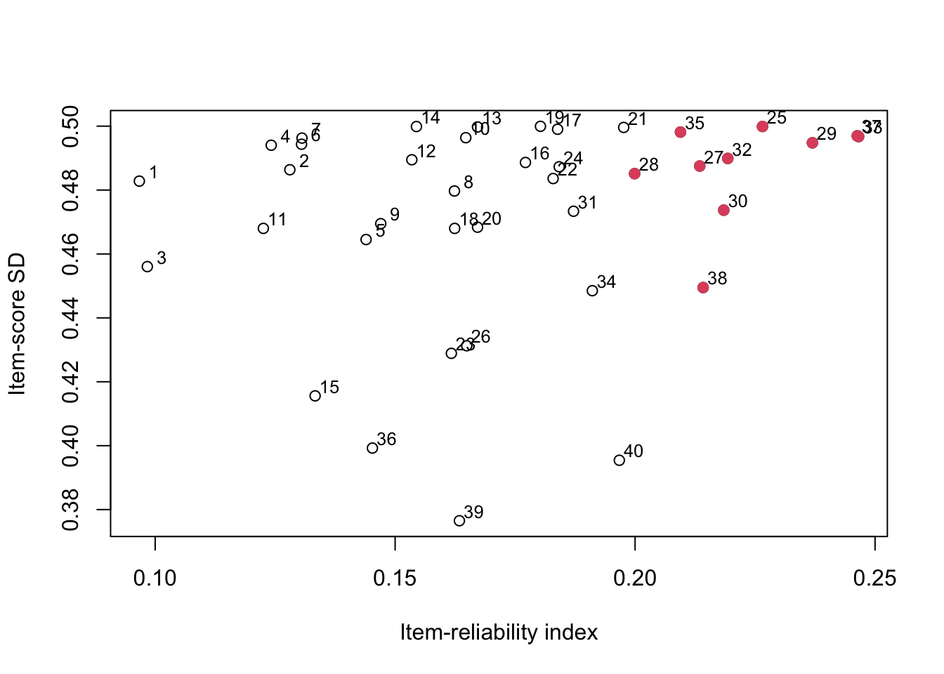
For example, just based on eyeballing here, these are:
33, 37, 29, 25, 32, 30, 27, 35, 28, 38
Let’s try to see which items have the largest \(s_{i}r_{iX}\):
##  [1] 33 37 29 25 32 30 38 27
##  [9] 35 28
Note: The order(, decreasing = TRUE) function ranks the values from largest to smallest. In other words, item 33 has largest \(s_ir_{iX}\), item 37 has second largest, etc.
Compared to the points on the right edge, we can see that points on the right edge are essentially the ones that maximize item reliability index.
In other words, to maximize internal consistency reliability of the 10-item test, you can select the top 10 questions with largest item reliability, \(s_ir_{iX}\).
8.2.2 Maximizing Validity Coefficient
To maximize the test validity for predicting \(Y\), Allen and Yen (1971) suggested plotting the item validity indices (y-axis) against item reliability indices (x-axis), and select the items appearing in the upper edge of the scatter plot.
# scatter plot for the item validity vs. item reliability index
plot(item_rel, item_val, xlab = "Item-reliability index", ylab = "Item-validity index")
text(item_rel + .003, item_val + .003, 1:40, cex = .8)
max_val <- order(item_val / item_rel, decreasing = TRUE)[1:10]
points(item_rel[max_val], item_val[max_val], col = 2, pch = 19)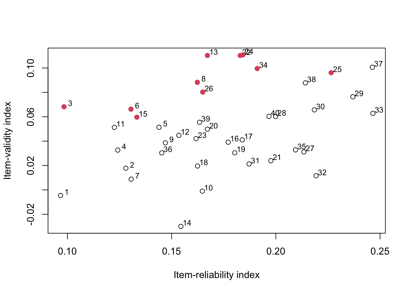
For example, just based on eyeballing here, these are:
13, 3, 22, 24, 8, 6, 11, 15, 26, 34
Let’s try to see which items have the largest \(\frac{s_ir_{iY}}{s_{i}r_{iX}}\):
##  [1]  3 13 22 24  8 34  6 26
##  [9] 15 25
We can see that points on the upper edge are essentially the ones that maximize the ratio between item validity and item reliability.
In other words, to maximize validity of the 10-item test for predicting criterion, you can select the top 10 questions with largest item validity-to-reliability ratio, \(\frac{s_ir_{iY}}{s_ir_{iX}}\).
8.2.3 Balancing Two Conflicting Objectives
Are there any overlapping items across these two?
We can use the intersect function to check this:
## [1] 25There is only one item, item 25, that was selected for both.
We want to design a test that is both reliable and valid. Sometimes, these two objectives are conflicting — items that maximize internal consistency not necessarily predict criterion score well, and vice versa.
If we want to balance these two objectives, we might want to assign weights to reliability and validity, and optimize the weighted average between these two objectives, i.e. \[w\cdot s_ir_{iX}+(1-w)\frac{s_{i}r_{iY}}{s_ir_{iX}}\]
Here, \(0\leq w\leq 1\). \(w\) represents the weight we give to reliability (intuitively, the amount of attention we give to reliability). The more attention/weight we give reliability, the smaller the \(1-w\), that is, we won’t be able to give much attention to validity.
Note that:
- When \(w = 1\), \(1 - w = 0\). The equation above equals \(s_ir_{iX}\). We select questions only based on reliability.
- When \(w = 0\), \(1 - w = 1\). The equation above equals \(\frac{s_ir_{iY}}{s_ir_{iX}}\). We select items that maximize validity only.
Below is the code for selecting items where we give reliability and validity equal weight of .5, i.e., \(w = .5\)
w <- .5

obj <- w * item_rel + (1 - w) * (item_val / item_rel)

max_weighted_both <- order(obj, decreasing = TRUE)[1:10]

max_weighted_both
## [1] 13 3 22 24 34 8 37 26
## [9] 25 6You can play with this and try different values of \(w\), e.g., \(0, .1, \ldots, .9, 1\). The 10-item test selected this way will be a balance between maximizing reliability and validity.