Random Variables
In this chapter, students will learn how to obtain some properties of probability distributions in R, such as the probability density, cumulative probability, and quantile. Three probability distributions will be discussed: binomial distribution, normal distribution, and uniform distribution. Students will be able to generate random samples from the probability distributions.
5.3 Binomial distribution
An experiment where there are only two possible outcomes, with probabilities of \(p\) and \(1-p\), is called a Bernoulli trial. An examples of Bernoulli trial is coin tosses. We can consider the result of getting heads as success and getting tails as failure. Another example is answering to a question, where the chance of correct answer is 40%. The outcomes of a Bernoulli trial follow a Bernoulli distribution with probability \(p\).
Now, suppose the Bernoulli trial is repeated \(n\) times. For example, answer to 10 questions, each with 40% chance of answering correctly. If \(x\) is the sum of the outcomes of the \(n\) repetitions, \(x\) follows a binomial distribution with \(n\) trials and probability \(p\).
The probability mass function of the binomial distribution is:
\[P(X=k) = {n \choose k} p^k (1-p)^{n-k}\]
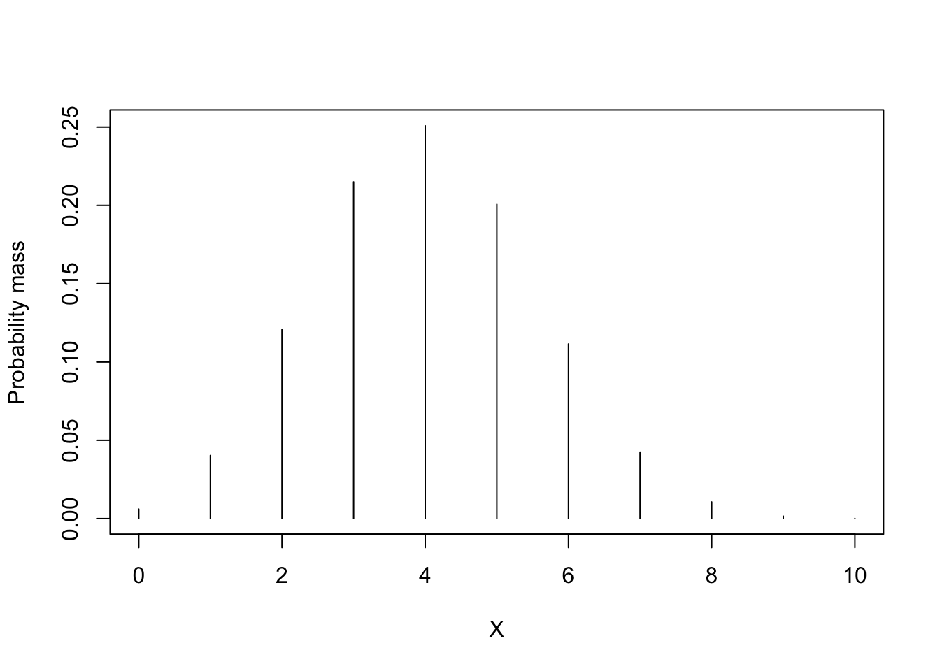
If a subject answers to \(n=10\) questions and the probability of correct response for each item is \(p=.4\), then the number of items that the subject correctly answers \(x\) follows a binomial distribution, \(Binom(10, .4)\).
This plot shows the probability mass function of a binomial distribution with \(n=10\) and \(p=.4\).
Let’s obtain the probability of getting exactly 5 items correct out of 10 items, with 40% chance of correct answer. You can use dbinom function to obtain the probability mass.
\[P(X = 5) = 0.201\]
## [1] 0.2006581The pbinom function returns the cumulative probability of a binomial distribution. The probability of correctly answering on 5 or less items out of 10 items, with \(p = .4\) is:
\[P(X \leq 5) = 0.8338\]
## [1] 0.8337614What is the 50% quantile of a binomial distribution with \(n=10\) and \(p=.4\)?
## [1] 4Let’s randomly draw 5 outcomes of Binomial(10, .4) trial.
## [1] 7 5 4 0 3Try to run the above code multiple times and compare the results. You will notice that every time you draw random samples, the same code gives different results. We can make the random samples replicable by setting the seed number. This can be useful when we want the results to be replicable by others.
## [1] 3 5 4 6 65.4 Normal distribution
The normal distribution is one of the commonly used continuous Random Variable in social sciences, especially when the underlying distribution of observations is unknown. The underlying ability/latent trait distribution of a population is often modeled using the normal distribution.
For example, the IQ scores in a population can follow a normal distribution with mean of 100 and sd of 10. The below plot shows the probability density of a normal distribution with mean of 100 and sd of 10, \(N(100, 10^2)\).
plot(50:150,
     dnorm(50:150, mean = 100, sd = 10),
     type = "l",
     xlab = "IQ",
     ylab = "Probability density")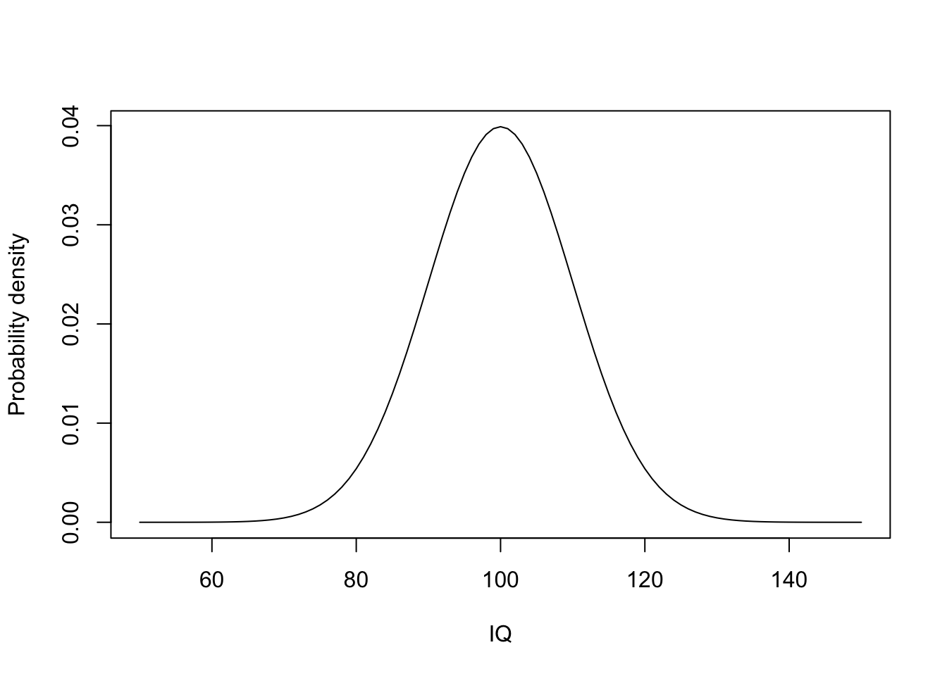
\[X \sim N(100, 10^2)\]
We can obtain the probability of getting a score of 120 or below using the pnorm() function.
\[P(X \leq 120)\]
## [1] 0.9772499Or we can obtain the probability of getting a score between 110 and 120 by:
\[P(110 \leq X \leq 120) = P(X \leq 120) - P(X \leq 110)\]
## [1] 0.1359051Let’s obtain the 90% quantile from the population IQ score.
## [1] 112.8155When we conduct simulation studies, we may assume the population of interest has standard normal latent ability distribution (i.e. N(0,1)). To generate 1000 subjects’ latent trait scores from this distribution, we can use
5.5 Uniform distribution
A Uniform random variable, U(\(a\), \(b\)), takes values between a and b, and the probability of getting any value between \(a\) and \(b\) is the same.
We often use the uniform distribution between 0 and 1, denoted \(U(0, 1)\).
It has the following properties:
- The probability density of any point between 0 and 1 is 1.
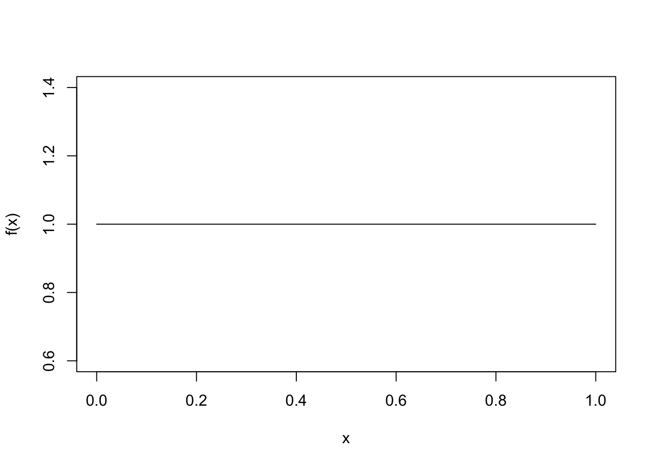
- The probability of getting a value less than or equal to \(p\) (between 0 and 1) is \(p\).
## [1] 0.3## [1] 0.7We can generate random numbers from the uniform distribution using runif() function:
## [1] 0.141085222 0.888621103
## [3] 0.008285004 0.569120653
## [5] 0.967550190## [1] 0.26918876 0.98396007
## [3] 0.03538949 0.25797643
## [5] 0.25989112## [1] 0.3896377 0.3959245
## [3] 0.3468770 0.2574960
## [5] 0.28179185.6 Your turn
Set your seed to
1234and randomly generate 100 values from the normal distribution \(N(50, 10^2)\). Save the generated samples and name it assamples.What is the proportion of the random samples that are greater than 60 and less than 80?
hint: (samples > 60 & samples < 80) will return a logical vector indicating whether each element of samples satisfies the condition or not.
- What is the theoretical probability of observing values greater than 60 and less than 80 from the above distribution?
hint: \(P(60 < X < 80) = P(X < 80) - P(X < 60)\)
- From a Bernoulli distribution with \(p = .5\), draw 10 random samples.
hint: The Bernoulli distribution is a special case of the binomial distribution where \(n = 1\).