Objects & Data Structure

1.9 Objects

Objects are very commonly used in R. We can create objects, store them in the environment, and use them later.

Let’s start with a motivating example: Suppose we are buying pumpkins and candy for Halloween. Each pumpkin costs 1.99 dollars. One bag of candy costs 4.99 dollars. We want to buy 5 pumpkins and one bag of candy. How much do we need to pay (before tax)?

One way is to calculate the whole thing with one equation:

5 * 1.99 + 4.99

## [1] 14.94

Another way would be to create and use objects:

cost_per_pumpkin <- 1.99

n_pumpkins <- 5

cost_bagcandy <- 4.99

# compute total cost
total <- n_pumpkins * cost_per_pumpkin + cost_bagcandy
# print total cost as output
print(total)

## [1] 14.94

Since our life (and statistics) is much more complex than buying pumpkins and candy, objects can come in handy when we cannot do everything within one equation. Objects are also helpful when we want to keep track of what our code is doing. For example, if you come back 1 week later to this code, you may not remember what 5*1.99+4.99 referred to, but n_pumpkins*cost_per_pumpkin+cost_bagcandy is quite self-explanatory.

Now, let’s take a closer look at cost_per_pumpkin <- 1.99:

Here, you created an object of value 1.99, and used <- to assign it to an object name, cost_per_pumpkin.
Keyboard shortcut for <-: Windows: Alt + -, Mac: Option+-. Could use = instead of <- but this is discouraged.
After running this line, you will see cost_per_pumpkin as an object in the Environment pane (topright.) Objects that show up in the environment can be referenced in your code. To remove an object from environment, use rm(), e.g., rm(cost_per_pumpkin).
The object name is just a label, so you can re-assign it with new values, e.g.:

# gas price in Jan 2022
gas_price <- 2.5

# gas price in March
gas_price <- 3.5
print(gas_price)

## [1] 3.5

# gas price in July increased by 50% 
gas_price <- gas_price * 1.5
print(gas_price)

## [1] 5.25

1.9.1 Naming an object

You have a lot of flexibility in how to name an object, but an object name needs to satisfy a few syntactic rules:

a name must consist of letters, digits, . and _, e.g.,

x.1 <- 1
y_1 <- 2

but it cannot start with _ or a digit, e.g.,

_x <- 1
#> Error: unexpected input in "_"

1.x <- 2
#> Error: unexpected symbol in "1.x"

and it cannot be some reserved special names, e.g., if, TRUE/FALSE, function:

if <- 3
#> Error: unexpected assignment in "if <-"

Lastly, R is case-sensitive, meaning that it treats upper- and lower-case characters as different characters. e.g., we created gas_price, but if you try calling Gas_price, you’ll get an error saying it is not found.

gas_price

## [1] 5.25

Gas_price
#> Error: object 'Gas_price' not found

1.10 Data structure

In R, the data that you analyze should be stored in the environment as objects. Now let’s talk about common types of data.

1.10.1 Scalars

The objects you have seen above, e.g., cost_per_pumpkin = 1.99, are scalars, i.e., individual values. There are 4 types of scalars:

Logicals:
- In full (TRUE or FALSE),
- Abbreviated (T or F).
Doubles:
- Decimal (0.1234), scientific (1.23e4, i.e., $1.23\times 10^4$)
- Special values unique to doubles: Inf ($\infty$), -Inf ($-\infty$), and NaN (not a number). e.g., try running 0/0 and see what you get.
Integers:
- Similar to doubles but
  - must be followed by L (1234L, 1e4L, or 0xcafeL),
  - and can not contain fractional values.
Strings:
- Surrounded by " (e.g., "hi"), or ', (e.g., 'bye').

Lastly, a special value, NA, represents missing value.

1.10.2 Vectors

Scalars serve as building blocks of a more complex type of object, vectors. You might recall from math that a vector is a 1-dimensional list with multiple elements, e.g., $(1,2,3)^\prime$ is a vector of length 3, whose first element is the scalar $1$. However, in R, vectors denote a more general collection of objects.

Depending on (1) the dimension of the object and (2) whether its elements are of the same type (e.g., all numeric), there are different types of vectors:

Vector	Homogeneous	Heterogeneous
1d	Atomic vector	List
2d	Matrix	Data frame
nd	Array	-

Almost all other objects are built upon these foundations.
Best way to understand what data structures any object is composed of is str() (short for structure).

An atomic vector, like the one below, is a 1-dimensional vector with length 4. The 4 elements are all doubles.

x <- c(5, 29, 13, 87)
str(x)

##  num [1:4] 5 29 13 87

Here, c() is the concatenate function, which can be used to create an atomic vector. Of course, you can also have atomic vectors containing all logical, integer, or strings, e.g.,

lgl_var <- c(TRUE, FALSE)
int_var <- c(1L, 6L, 10L)
dbl_var <- c(1, 2.5, 4.5)
chr_var <- c("these are", "some strings")

Now, suppose you see an object called lgl_var in your environment, but you don’t know what it is. There are a few functions that come in handy for checking what it is: str(), typeof(), class():

str(lgl_var)

##  logi [1:2] TRUE FALSE

typeof(lgl_var)

## [1] "logical"

class(lgl_var)

## [1] "logical"

Here class() and typeof() give you the same output, the difference being typeof() cannot be modified, but you can change class(lgl_var) to something else you like, e.g., "cat".

You can also use the c() function to combine two vectors - this creates a long 1d vector:

c(c(1, 2), c(3, 4))

## [1] 1 2 3 4

Often, we encounter missing values in a data set, e.g., for a class of 8 students, we want to know what year everyone is, but one student missed the class and didn’t respond. In this case, NA can be an element of a data vector representing missingness:

# student year in a 8-student class. Student 3 didn't respond:
year <- c(2, 4, NA, 3, 3, 1, 3, 4)

# check the length of a vector
length(year)

## [1] 8

Now you may ask, what would happen if I create a vector containing scalars of different types?

mixed_vec <- c('apple', 2.5, TRUE)

str(mixed_vec)

##  chr [1:3] "apple" "2.5" ...

Recall that an atomic vector (created with c()) must contain homogeneous elements. When combining different types, coercion happens, in a fixed order (character $\to$ double $\to$ integer $\to$ logical). In other words, if your elements contain characters, everything will be coerced into a character. In the example above, TRUE (logical) and 2.5 (double) both were converted to characters wrapped in quotes, a character of "TRUE", and another of "2.5".

You can also coerce an object into a different type using as.() functions, for instance, as.numeric() coerces an object into numeric type:

# a length-3 logical vector
x <- c(TRUE, TRUE, FALSE)
as.numeric(x)

## [1] 1 1 0

But if a value cannot be coerced into another type, NAs will be introduced:

# a character vector
y <- c('1.8', '3', 'cat')
as.integer(y)

## Warning: NAs introduced by
## coercion

## [1]  1  3 NA

So what if you need to create a vector, containing heterogeneous objects? In this case, instead of creating an atomic vector using c(), you can create a list.

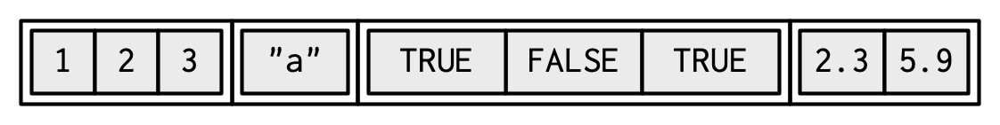
A list is a heterogeneous 1d vector. Each element can be of a different type. In addition, the elements don’t necessarily need to be scalars. For example, it can be an atomic vector of length 3. To create a list, we use the list() function:

l1 <- list(
  1:3,
  "a",
  c(TRUE, FALSE, TRUE),
  c(2.3, 5.9)
)
typeof(l1)

## [1] "list"

str(l1)

## List of 4
##  $ : int [1:3] 1 2 3
##  $ : chr "a"
##  $ : logi [1:3] TRUE FALSE TRUE
##  $ : num [1:2] 2.3 5.9

As str() informs us, l1 is a list of 4 elements:

First element is a length-3 vector, 1:3, or equivalently, c(1,2,3)
Second element is a character scalar, a
Third element is a logical vector of length 3, c(TRUE, FALSE, TRUE)
Fourth element is a length-2 numeric vector, c(2.3, 5.9).

This is equivalent to:

# create individual elements first
e1 <-  1:3
e2 <-  "a"
e3 <-  c(TRUE, FALSE, TRUE)
e4 <- c(2.3, 5.9)

# combind them to list
l1 <- list(
  e1, e2, e3, e4
)

str(l1)

## List of 4
##  $ : int [1:3] 1 2 3
##  $ : chr "a"
##  $ : logi [1:3] TRUE FALSE TRUE
##  $ : num [1:2] 2.3 5.9

The figure below represents the structure of this list, think of it as a train with 4 carriages, inside each carriages are more individual elements.

You can also give names to each element of a list, e.g.,

l2 <- list(
  fruits = c('apple', 'orange'),
  rooms = 1:5
)

str(l2)

## List of 2
##  $ fruits: chr [1:2] "apple" "orange"
##  $ rooms : int [1:5] 1 2 3 4 5

1.10.3 Subsetting

There are 2d and n-dimensional objects, e.g., matrices, data frames. We will talk about them later when we strat playing with data sets. Now, let’s use 1d vectors to introduce subsetting.

Let’s start with a simple case. For the year vector above (8 students’ year):

# the original year vector
year

## [1]  2  4 NA  3  3  1  3  4

The 3rd student came to the next class and told the teacher that he is in year 2. How can we modify the year vector to update its 3rd entry? We can use [] to refer to entries (or a single entry) of an atomic vector:

# this subsets the 3rd entry of year
year[3]

## [1] NA

# this subsets the 1st to 3rd entries of year
year[1:3]

## [1]  2  4 NA

# this subsets the 1st and the 3rd entries of year
year[c(1,3)]

## [1]  2 NA

Now, to change the value of year[3], we use the <- learned earlier. Code below assigns the value 2 to the 3rd element of year:

year[3] <- 2

Now let’s look at year again:

year

## [1] 2 4 2 3 3 1 3 4

To subset a list, we make use of [[]] to refer to a specific element, and [] to a subset. Consider the following list:

x <- list(1:3, "a", 4:6)

str(x)

## List of 3
##  $ : int [1:3] 1 2 3
##  $ : chr "a"
##  $ : int [1:3] 4 5 6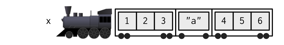

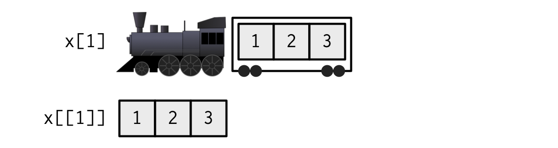
When extracting a single element, you have two options:
- Create a smaller train, i.e., fewer carriages, with [.
- Extract the contents of a particular carriage with [[.

When extracting multiple (or even zero!) elements, you have to make a smaller train.

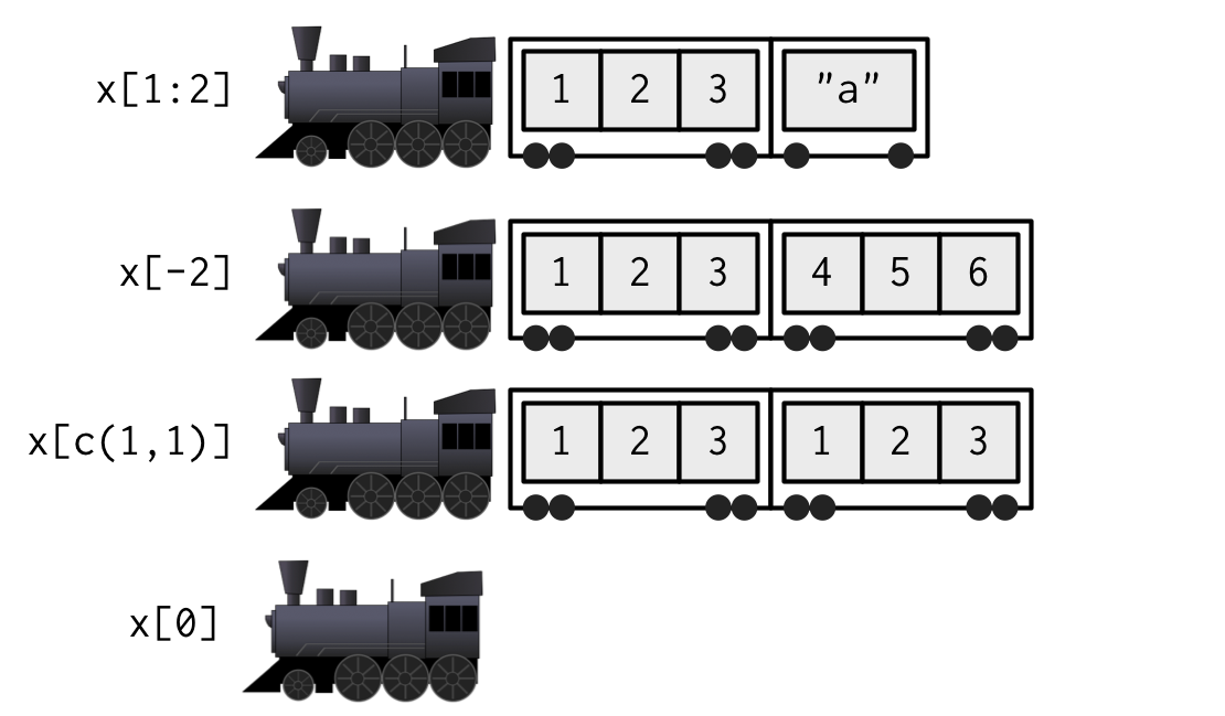
You can also subset recursively, e.g., to get the “2” (2nd element) from the first list element:

x[[1]][2]

## [1] 2

To refer to a specific element of a named list, use $:

l2$fruits

## [1] "apple"  "orange"

1.11 Your turn

As an exercise, try writing the R code for each problem below. At the end you’ll create something that looks like a receipt from grocery purchase.

Create a character vector called Item, containing four character elements, “milk”, “cold brew coffee”, “dishliquid”, and “avocado”.
Create a numeric vector called Unit_price, containing the price of each item, 3.9, 6, 1.5, 1.
Create an integer vector called Quantity, containing the purchased quantity of each item, 1, 1, 1, 4.
Now let’s calculate the total cost on each item, try multiplying Unit_price with Quantity, assign it the name Cost, use str() to check the structure of Cost. What do you think * does?
The sum() function computes the sum of all elements of an input vector, and call it Total. Use it to figure out the total cost for purchasing all 4 items.
Create a list called receipt, containing Item, Unit_price, Quantity, Cost, and Total as its 5 elements.
From the receipt list, can you subset it to get the unit price, quantity, and total cost spent on avocados?

1.12 A peak into next time:

You might have noticed, it is not straightforward to subset all entries corresponding to avocados. A more efficient way of storing a data set is as a data.frame, i.e., a 2d heterogeneous object. In this case, the data set will be rectangular, each row being a case (here, milk, coffee, dishliquid, avocado), and columns represent different variables that describe the case (e.g., unit price, quantity bought, total cost).

More on matrix and data frames next time.
Next week, we’ll also talk about control flows (e.g., if, for loop etc.)