Scaling
Scores are considered to have equal intervals if any given difference between scores always represents the same amount of difference in the trait being measured. Equal interval scales are useful for studying growth or change in a trait. However, not all raw scores are equal-interval. We can transform a set of raw scores to an equal interval scale by the normalization method discussed in the previous chapter.
9.4 Thurstone’s Absolute Scaling Method
Thrustone’s absolute scaling method is commonly used for constructing an equal interval scale. There are two assumptions of this method:
The measured trait is continuous and has a normal distribution in some specified population.
The raw scores on the test are monotonically related to the trait values.
If the two assumptions are satisfied, then the normalized scores will have equal intervals. We can verify if the scales are actually equal-interval by plotting the two normalized scores from the two samples.
Step 1: Administer the test to two samples of examinees, each assumed to have a normal distribution of trait values.
Step 2: Normalize the raw scores within each sample. (e.g., z-scores or T-scores)
Step 3: If these two sets of normalized scores are linearly related, then the normalized test scores obtained from either sample form an equal-interval scale.
As an illustration, we are going to use the following data set. You can download the attached “equating.RData” file below and import the file into your RStudio using the load() function.
eqauting.RData: Download
The two objects X1 and X2 are the raw scores on the same test from two different samples. Let’s construct frequency tables for both samples.
freq_table1 <- cbind(as.numeric(names(freq1)),
                     freq1,
                     cumsum(table(X1)))
freq_table2 <- cbind(as.numeric(names(freq2)),
                     freq2,
                     cumsum(table(X2)))
colnames(freq_table1) <- colnames(freq_table2) <- c("Scores", "Freq", "CumFreq")
freq_table1
## Scores Freq CumFreq
## 0 0 4 4
## 1 1 10 14
## 2 2 18 32
## 3 3 30 62
## 4 4 38 100
## 5 5 38 138
## 6 6 30 168
## 7 7 18 186
## 8 8 10 196
## 9 9 2 198
## 10 10 2 200## Scores Freq CumFreq
## 0 0 4 4
## 1 1 6 10
## 2 2 8 18
## 3 3 14 32
## 4 4 18 50
## 5 5 24 74
## 6 6 26 100
## 7 7 26 126
## 8 8 24 150
## 9 9 18 168
## 10 10 14 182
## 11 11 8 190
## 12 12 10 200Percentile scores from X1:
scores1 <- min(X1):max(X1)
percentiles1 <- numeric(length(scores1))
for(i in 1:length(scores1)) {
  score <- scores1[i]
  below_num1 <- freq_table1[which(freq_table1[, 1] == score), 3] - freq_table1[which(freq_table1[, 1] == score), 2] / 2
  percentiles1[i] <- below_num1 / length(X1) * 100
}
Percentile scores from X2:
scores2 <- min(X2):max(X2)
percentiles2 <- numeric(length(scores2))
for(i in 1:length(scores2)) {
  score <- scores2[i]
  below_num2 <- freq_table2[which(freq_table2[, 1] == score), 3] - freq_table2[which(freq_table2[, 1] == score), 2] / 2
  percentiles2[i] <- below_num2 / length(X2) * 100
}
percentiles2
## [1] 1.0 3.5 7.0 12.5 20.5
## [6] 31.0 43.5 56.5 69.0 79.5
## [11] 87.5 93.0 97.5## scores1 percentiles1
## [1,] 0 1.0
## [2,] 1 4.5
## [3,] 2 11.5
## [4,] 3 23.5
## [5,] 4 40.5
## [6,] 5 59.5
## [7,] 6 76.5
## [8,] 7 88.5
## [9,] 8 95.5
## [10,] 9 98.5
## [11,] 10 99.5## scores2 percentiles2
## [1,] 0 1.0
## [2,] 1 3.5
## [3,] 2 7.0
## [4,] 3 12.5
## [5,] 4 20.5
## [6,] 5 31.0
## [7,] 6 43.5
## [8,] 7 56.5
## [9,] 8 69.0
## [10,] 9 79.5
## [11,] 10 87.5
## [12,] 11 93.0
## [13,] 12 97.5We can now obtain the normalized z-scores using qnorm().
Below, each table shows the percentiles and the normalized z_scores corresponding to the raw scores.
##       scores1 percentiles1
##  [1,]       0          1.0
##  [2,]       1          4.5
##  [3,]       2         11.5
##  [4,]       3         23.5
##  [5,]       4         40.5
##  [6,]       5         59.5
##  [7,]       6         76.5
##  [8,]       7         88.5
##  [9,]       8         95.5
## [10,]       9         98.5
## [11,]      10         99.5
## z_score1
## [1,] -2.3263479
## [2,] -1.6953977
## [3,] -1.2003589
## [4,] -0.7224791
## [5,] -0.2404260
## [6,] 0.2404260
## [7,] 0.7224791
## [8,] 1.2003589
## [9,] 1.6953977
## [10,] 2.1700904
## [11,] 2.5758293## scores2 percentiles2
## [1,] 0 1.0
## [2,] 1 3.5
## [3,] 2 7.0
## [4,] 3 12.5
## [5,] 4 20.5
## [6,] 5 31.0
## [7,] 6 43.5
## [8,] 7 56.5
## [9,] 8 69.0
## [10,] 9 79.5
## [11,] 10 87.5
## [12,] 11 93.0
## [13,] 12 97.5
## z_score2
## [1,] -2.3263479
## [2,] -1.8119107
## [3,] -1.4757910
## [4,] -1.1503494
## [5,] -0.8238936
## [6,] -0.4958503
## [7,] -0.1636585
## [8,] 0.1636585
## [9,] 0.4958503
## [10,] 0.8238936
## [11,] 1.1503494
## [12,] 1.4757910
## [13,] 1.9599640Plot the two z-scores and check if it is a straight line.
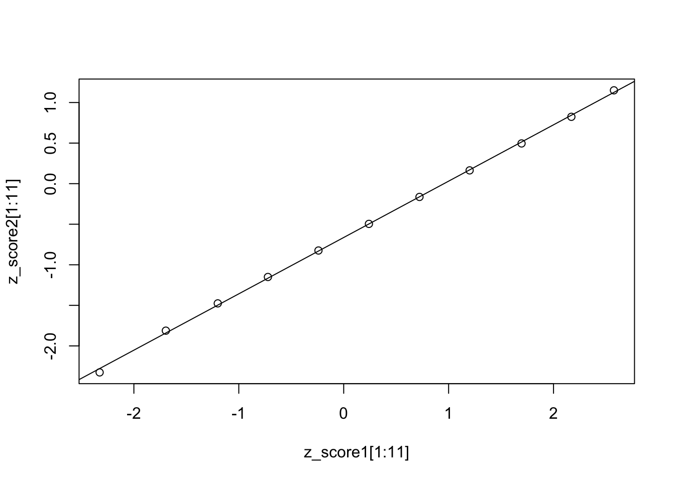
The plot verifies that either Z is approximately equal-interval.