Week 11 Item Response Theory 2
In the last chapter, we generated random response data resp for 1,000 examinees on the 40 items from GRE40. We are going to continue to use the resp response data set. The following code will generate resp.
GRE40 <- read.table("https://raw.githubusercontent.com/sunbeomk/PSYC490/main/GRE40.txt")

# IRF
irt_p <- function(theta, a, b, c){
  p <- c + (1-c) / (1 + exp(-1.7 * a * (theta - b)))
  p
}

set.seed(123) # set the random seed
theta_sim <- rnorm(1000) # true ability thetas
n_subjects <- 1000
n_items <- 40
resp <- matrix(NA, n_subjects, n_items)
for (i in 1:n_subjects) {
  for (j in 1:n_items) {
    pij <- irt_p(theta_sim[i], GRE40$a[j], GRE40$b[j], GRE40$c[j])
    resp[i, j] <- rbinom(1, 1, prob = pij)
  }
}

dim(resp)
## [1] 1000 40In practice, after administering the test, the only thing we get might be resp. That is, we do not know the true \(\theta\)s (theta_sim). In this chapter, students will use this resp data set to draw an empirical ICC plot and to estimate individuals’ \(\theta\)s. We will use an R package mirt to estimate the item parameters of IRT models.
11.1 Empirical ICC
Item characteristic curve (ICC) is a graphic representation of probability (or proportion) of answering an item correctly by the tested construct values (total score or \(\theta\)).
- If \(x-\)axis is latent trait (\(\theta\)) and \(y-\)axis is the probability of correct response calculated from IRF, it gives the theoretical ICC.
- If \(x-\)axis is total score (\(X\)) and \(y-\)axis is the proportion of correct response computed from subsample, it gives the empirical ICC.
Empirical ICC is useful when you don’t know the IRF and the true \(\theta\)s.
Drawing the empirical ICC involves a few steps:
- Bin individuals based on their total scores (e.g., 2-4, 4-6, 6-8, …)
- Compute the percent correct on item \(j\) in each total score bin. (e.g., \(\%\) correct in 2-4, \(\%\) correct in 4-6, \(\ldots\))
- Plot \(\%\) correct against average score of each bin.
Let’s work with resp. Suppose we want to draw the ICC of item 1.
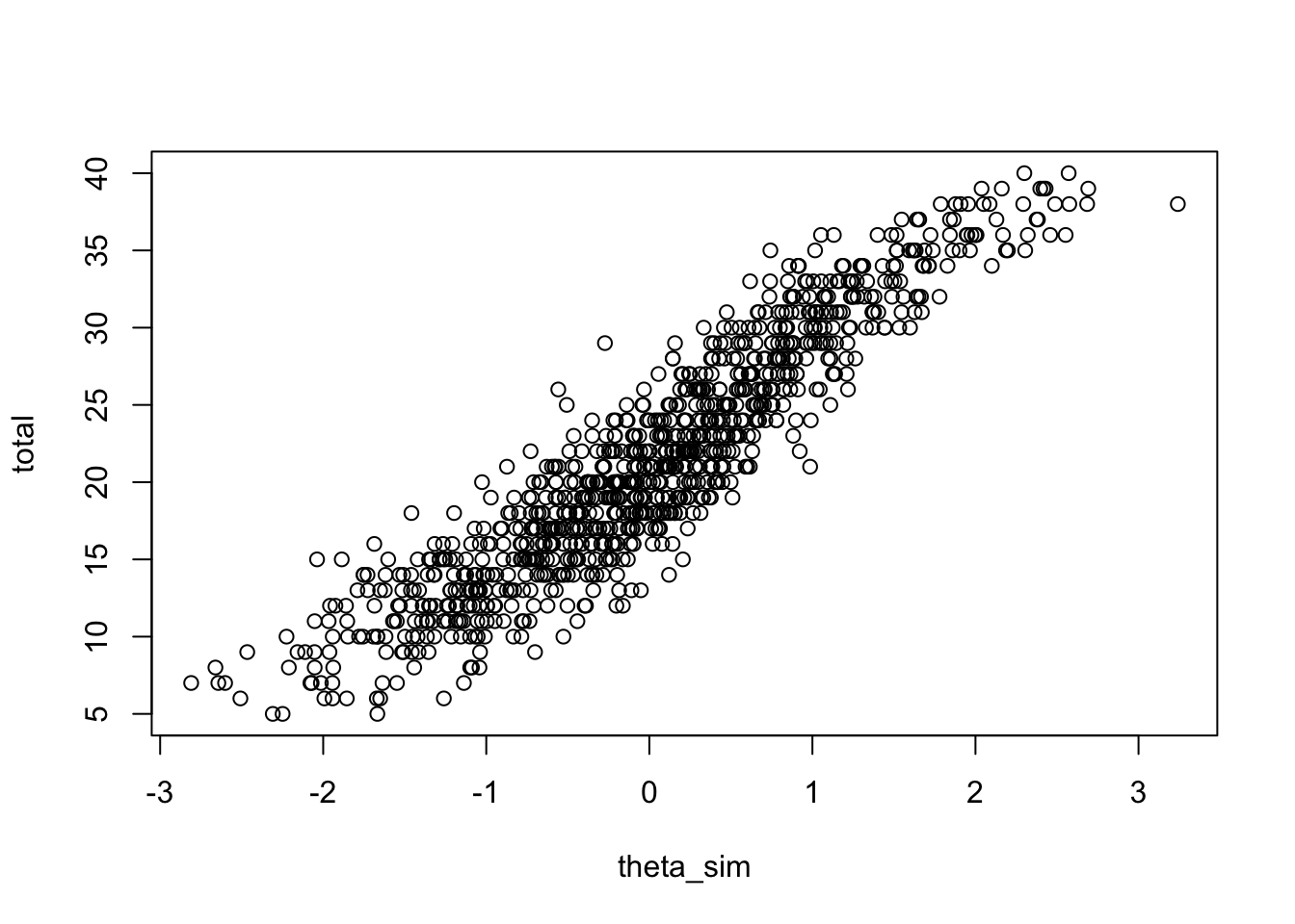
Step 1: Get total scores
Step 2: Find proportion correct in each score interval
Step 3: Drawing
11.1.2 Step2: Find proportion correct in each score interval
For drawing ICC, we want to find out the % correct of item 1 in each interval of total score.
The total score on a 40-item test ranges between 0 and 40. So we will bin people into equally spaced total score intervals, ranging from \(0\) to \(40\). To ensure sufficient people in each interval, let us use bin size of 2. Thus the bins will be
- [0,2)
- [2,4)
- …
- [38,40)
- [40,42) (for exact score \(40\))
We will create a matrix with 3 columns:
- Median score in bin (e.g., for 1-2, median is 1.5)
- Number of examinees (e.g., how many test takers got score between 1 and 2)
- Number answered correctly (e.g., how many test takers in this bin answered right on item 1)
The code below uses a for() loop to create this matrix.
# specify item index
j = 1 # 1st item out of 40.


# create sequence of cut points for binning
scores <- seq(0, 40+2, 2) # 42 because we want a last bin between [40,42)

# empty matrix of NAs
score_bin_mat <- matrix(NA, (length(scores) - 1), 3)

# for each score interval
for(i in 1:(length(scores) - 1)){
  # first column: median
  score_bin_mat[i, 1] <-  scores[i] + 1
  # second column: total number of people
  score_bin_mat[i, 2] <- sum(total >= scores[i] & total < (scores[i + 1]))
  # third column: number of people answering correctly in this bin
  score_bin_mat[i, 3] <- sum(resp[which(total >= scores[i] & total < (scores[i + 1])), j])
}

# give columns names
colnames(score_bin_mat) <- c("Med.Score", "# Test Takers", "# Correct")

score_bin_mat
## Med.Score # Test Takers
## [1,] 1 0
## [2,] 3 0
## [3,] 5 3
## [4,] 7 17
## [5,] 9 21
## [6,] 11 50
## [7,] 13 67
## [8,] 15 85
## [9,] 17 91
## [10,] 19 104
## [11,] 21 107
## [12,] 23 85
## [13,] 25 70
## [14,] 27 64
## [15,] 29 56
## [16,] 31 56
## [17,] 33 44
## [18,] 35 35
## [19,] 37 26
## [20,] 39 17
## [21,] 41 2
## # Correct
## [1,] 0
## [2,] 0
## [3,] 1
## [4,] 5
## [5,] 6
## [6,] 26
## [7,] 27
## [8,] 47
## [9,] 51
## [10,] 62
## [11,] 69
## [12,] 55
## [13,] 50
## [14,] 52
## [15,] 40
## [16,] 42
## [17,] 37
## [18,] 25
## [19,] 22
## [20,] 16
## [21,] 2We can use this info to compute % correct rate in each score bin. Note that some bins have no one inside. We substitute the NANs by NA (missing).
##  [1]       NaN       NaN
##  [3] 0.3333333 0.2941176
##  [5] 0.2857143 0.5200000
##  [7] 0.4029851 0.5529412
##  [9] 0.5604396 0.5961538
## [11] 0.6448598 0.6470588
## [13] 0.7142857 0.8125000
## [15] 0.7142857 0.7500000
## [17] 0.8409091 0.7142857
## [19] 0.8461538 0.9411765
## [21] 1.0000000## [1] NA NA
## [3] 0.3333333 0.2941176
## [5] 0.2857143 0.5200000
## [7] 0.4029851 0.5529412
## [9] 0.5604396 0.5961538
## [11] 0.6448598 0.6470588
## [13] 0.7142857 0.8125000
## [15] 0.7142857 0.7500000
## [17] 0.8409091 0.7142857
## [19] 0.8461538 0.9411765
## [21] 1.0000000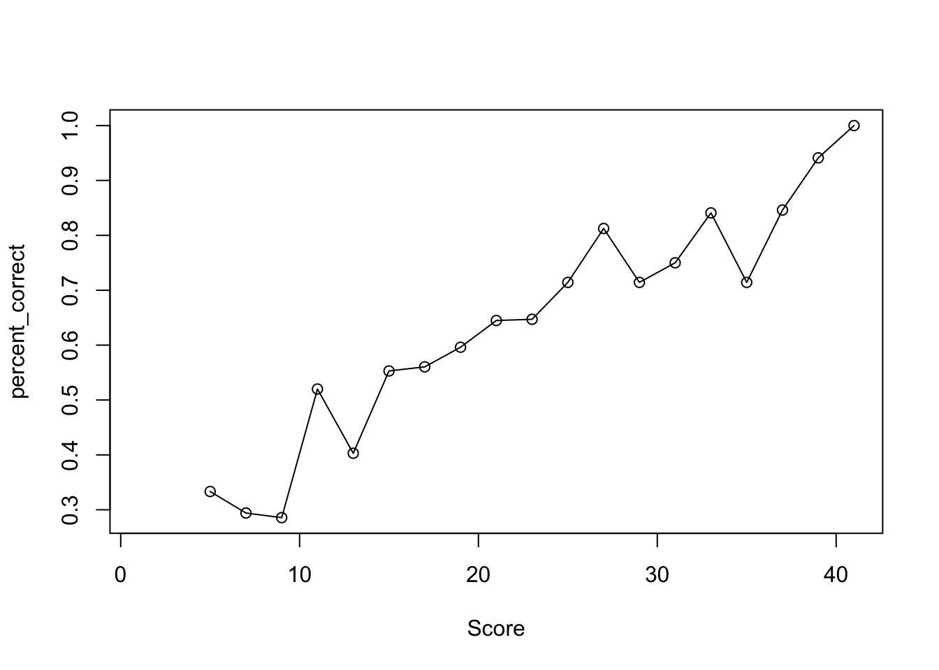
11.2 IRT ability (\(\theta\)) estimation
Suppose that now we know the GRE40 item parameters and know the responses of 1000 individuals - resp. However, we do not know their true abilities. How can we estimate their true ability? We can use the conditional Maximum likelihood estimation to estimate the ability \(\theta\) for all examinees, denoted \(\hat\theta\). Let’s do this on the resp data and find the 1000 examinees estimated \(\theta\)s using MLE.
The log likelihood function for examinee \(i\) is given by:
\[ \log L(\theta_i; \boldsymbol{Y_i}) = \log[\prod_{j=1}^J P(Y_{ij}\mid\theta_i)] =\sum_{j=1}^J \log[ P(Y_{ij}\mid\theta_i)].\]
The function below computes the likelihood of a response vector (\(Y_{i1}, \ldots, Y_{i,40}\)).
# loglikelihood function
loglike <- function(theta,     # a scalar of theta
                    a, b, c,      # vectors of a,b,c
                    response) {  # a scalar or a vector of dichotomous response
  p <- irt_p(theta, a, b, c)
  loglike <- sum(log(p) * response + log(1 - p) * (1 - response))

  loglike
}
What we want to do is, given a person \(i\)’s responses and the GRE40 a,b,c parameters, find out what \(\theta\) can make loglike the largest.
The below function implements this.
# function that computes mle by optimizing loglikelihood
MLE_theta <- function(a,b,c,
response, # a scalar or a vector of dichotomous response
max_est, # maximum estimate given to all-correct response
min_est){ # minimum estimate given to all-incorrect response
if (sum(response) == length(response)){
estimate <- max_est
}
else if (sum(response) == 0){
estimate <- min_est
}
else{
estimate <- optimize(loglike,
interval = c(min_est, max_est),
maximum = TRUE,
a = a,
b = b,
c = c,
response = response)$max
}
estimate
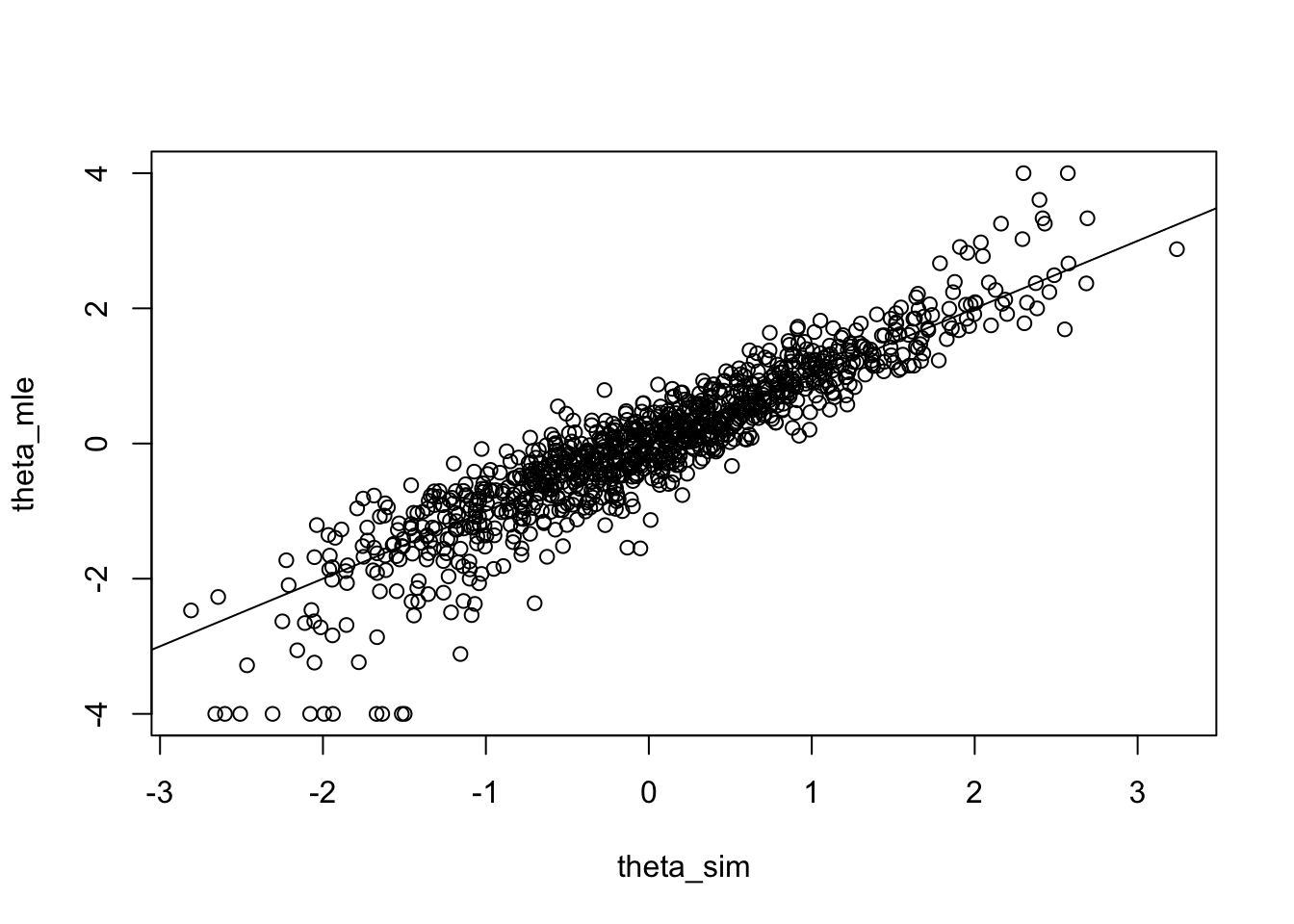
}Here, we set max_est and min_est, which are the maximum and mimimum possible \(\hat\theta\)s. For those who answer all questions correctly/incorrectly, \(\hat\theta\) will be set to these maximum/minimums. Commonly used options include
max_est = 4 and min_est = -4.
Let’s try to use this function to calculate \(1000\) examinees’ estimated ability.
# first create an empty vector
theta_mle <- numeric(1000)

# replace 0s by estimated theta
for (i in 1:1000) {
  theta_mle[i] <- MLE_theta(a = GRE40$a,
                            b = GRE40$b,
                            c = GRE40$c,
                            response = resp[i, ],
                            min_est = -4, max_est = 4)
}
Let us take a look and see how the true thetas (theta_sim) and estimates (theta.mle) relate.
11.3 IRT item parameter estimation
We have estimated the ability \(\theta\) assuming that we know the true item parameters. This time, however, we assume that we know even less. We have collected response data (resp). By plotting the empirical ICCs, we think the items follow 3PL model. However, we do NOT know either the item parameters (\(a,b,c\)) or the examinees’ abilities (\(\theta\)).
Our goal is using the resp data to estimate \(a_j, b_j, c_j\) for each item \(j\) and \(\theta_i\) for each examinee \(i\) simultaneously.
We will illustrate one method to simultaneously estimate \(a,b,c\) and \(\theta\)s. Specifically, it involves two parts:
Part 1: Estimate item parameters by marginal maximum likelihood estimation (MMLE). In other words, we integrate out \(\theta\)s from the likelihood to get the marginal likelihood of item parameters.
Part 2: Treat the estimated item parameters as known. Now that we know the responses and the \(\hat a, \hat b ,\hat c\)s for each item, we can estimate latent \(\theta\)s using CMLE (just like last time).
11.3.1 Part 1: Estimate item parameters by MMLE.
\[L(\boldsymbol{a},\boldsymbol{b}, \boldsymbol{c}; \boldsymbol{Y}) = \prod_{i=1}^N \left\{\int \prod_{j=1}^J P(Y_{ij}\mid\theta)f(\theta)d\theta\right\},\] where \(f(\theta)\) is the assumed density of \(\theta\) (e.g., \(N(0,1)\)). Then, we find values of \(\boldsymbol{a} = (a_1, \ldots, a_J), \boldsymbol{b} = (b_1, \ldots, b_J), \boldsymbol{c} = (c_1,\ldots, c_J)\) that maximize \(L(\boldsymbol{a},\boldsymbol{b}, \boldsymbol{c}; \boldsymbol{Y})\). The \(\boldsymbol{a}, \boldsymbol{b}, \boldsymbol{c}\) values that maximize the marginal likelihood will be the MML estimates of the item parameters. Denote the \(j\)th item’s parameter estimates by \(\hat a_j, \hat b_j, \hat c_j\). In practice, we sometimes call this step item calibration (synonym to item parameter estimation). The item parameters can be saved for later use.
For this part, we are going to use the mirt package.
Inside the mirt package, there is a mirt() function (yep they have the same names) that performs item parameter estimation. This is actually a very sophisticated and flexible function. For example, aside from estimating 3PL item parameters using marginal maximum likelihood, it can also do some of the following:
- Estimate item parameters with other methods (e.g., Bayesian)
- Estimate parameters for polytomous items (e.g., graded response model)
- Fit multidimensional IRT models
- Fit unfolding/ideal point IRT models (e.g., GGUM)
Here is the manual to the mirt package: mirt package manual
The full description to the mirt() function starts on page 100. A list of models it fits is described starting page 111. You can also type ?mirt in R and get the same documentations. It might be less as pretty and easy-to-read, though.
Running the mirt() function will require you to give a name to each item. We do this by giving the resp matrix column names.
##  [1] "item_1"  "item_2"
##  [3] "item_3"  "item_4"
##  [5] "item_5"  "item_6"
##  [7] "item_7"  "item_8"
##  [9] "item_9"  "item_10"
## [11] "item_11" "item_12"
## [13] "item_13" "item_14"
## [15] "item_15" "item_16"
## [17] "item_17" "item_18"
## [19] "item_19" "item_20"
## [21] "item_21" "item_22"
## [23] "item_23" "item_24"
## [25] "item_25" "item_26"
## [27] "item_27" "item_28"
## [29] "item_29" "item_30"
## [31] "item_31" "item_32"
## [33] "item_33" "item_34"
## [35] "item_35" "item_36"
## [37] "item_37" "item_38"
## [39] "item_39" "item_40"
For fitting the 3PL model, the command we will use is actually quite simple:
## EM cycles terminated after 500 iterations.Here, we specified 3 inputs:
data: The data set we use,resp.model:1means that we will estimate the IRT model with1dimension (i.e., \(\theta\) is unidimensional)itemtype:3PLindicates that the item follows the 3 parameter logistic model. If you want to fit the 2PL instead (no guessing), replace with2PL.
The output of the mirt() function, est, is a very large object with lots of information. However, right now we only want the item parameters.
To extract the estimated item parameters, we use a method called coef(). Here we feed the mirt() output, est, into the coef() function. It returns a list with three elements.
##                 a           b
## item_1  0.5138663 -0.97069204
## item_2  0.8258378  1.05838024
## item_3  0.6470903 -2.69714171
## item_4  0.9231509 -0.42530666
## item_5  0.9430637 -1.70312015
## item_6  1.2715428  0.80481143
## item_7  0.9041134  0.42088271
## item_8  1.0128339  0.98718559
## item_9  1.2772358  1.19603764
## item_10 1.3245819 -0.23773947
## item_11 0.8532851 -1.88082128
## item_12 1.0577224 -1.20282380
## item_13 1.4639584  0.19155141
## item_14 0.7694606 -1.48479993
## item_15 1.1629014 -1.68174473
## item_16 1.3697704 -0.27866608
## item_17 1.1567427 -0.63374361
## item_18 1.8797279  1.24783977
## item_19 1.5948074 -0.07544239
## item_20 1.6210566  0.93635725
## item_21 1.3447848 -0.06464766
## item_22 1.3572364 -0.81600148
## item_23 1.7659200  1.36178955
## item_24 1.8066562  0.66243368
## item_25 1.3077928 -0.60616068
## item_26 1.8505119  1.17487888
## item_27 1.3306714  0.61963228
## item_28 1.6326750 -0.88083885
## item_29 2.1943139  0.23813964
## item_30 1.6618387  0.63465322
## item_31 2.0322691  0.65097199
## item_32 1.8940278  0.42312904
## item_33 1.5218339  0.26373887
## item_34 2.0946687  1.06978143
## item_35 2.3581284  0.23530414
## item_36 1.8599400  1.27565490
## item_37 2.8556768  0.23132252
## item_38 4.4523151  0.94237960
## item_39 2.2503703  1.52906050
## item_40 2.7173919  1.27713364
##                   g u
## item_1  0.050727234 1
## item_2  0.143841111 1
## item_3  0.031205935 1
## item_4  0.005336232 1
## item_5  0.006244853 1
## item_6  0.096723496 1
## item_7  0.126039827 1
## item_8  0.041735758 1
## item_9  0.249178698 1
## item_10 0.335267039 1
## item_11 0.019843711 1
## item_12 0.011497287 1
## item_13 0.239540787 1
## item_14 0.028404514 1
## item_15 0.135961535 1
## item_16 0.101089882 1
## item_17 0.026404673 1
## item_18 0.312956622 1
## item_19 0.287694926 1
## item_20 0.156175058 1
## item_21 0.199334623 1
## item_22 0.002466547 1
## item_23 0.044147123 1
## item_24 0.199963894 1
## item_25 0.008640883 1
## item_26 0.029902502 1
## item_27 0.227324329 1
## item_28 0.015643067 1
## item_29 0.068331285 1
## item_30 0.159923205 1
## item_31 0.106655566 1
## item_32 0.090327396 1
## item_33 0.259417204 1
## item_34 0.065858322 1
## item_35 0.181265116 1
## item_36 0.295771943 1
## item_37 0.483194477 1
## item_38 0.404871536 1
## item_39 0.158060194 1
## item_40 0.240429993 1
Using the code chunk below, create 3 vectors, a.est, b.est, c.est, representing the \(a,b,c\) estimates for the GRE40 items.
Let us compare them to the true values in the GRE40 data frame.
par(mfrow=c(1, 3))
# a parameters
plot(GRE40$a, a_est)
abline(0, 1)
# b parameters
plot(GRE40$b, b_est)
abline(0, 1)
# c parameters
plot(GRE40$c, c_est)
abline(0, 1)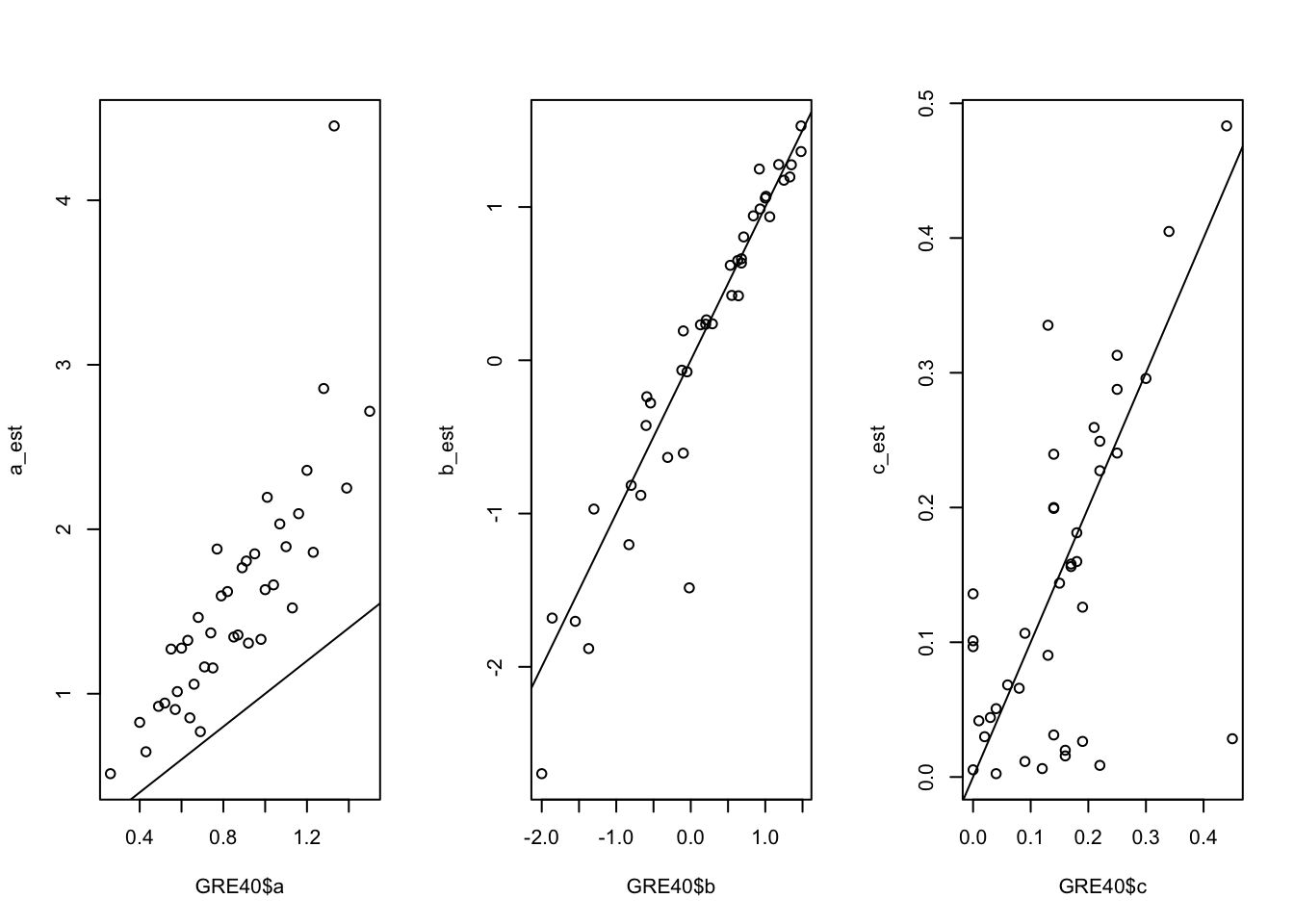
11.4 Information Function
11.4.1 Item Information Function
Item information function quantifies the amount of information in the data about \(\theta\). In IRT models, the item information function can be simplified as:
1PL: \(FI_j(\theta) = D^2P_j(\theta)Q_j(\theta)\)
2PL: \(FI_j(\theta) = D^2a_j^2P_j(\theta)Q_j(\theta)\)
3PL: \(FI_j(\theta) = \frac{D^2 a_j^2 Q_j(\theta) (P_j(\theta)-c_j)^2}{P_j(\theta)(1-c_j)^2}\)
where,
- \(P_j(\theta)\) : probability of correct response on item \(j\), given ability \(\theta\).
- \(b_j:\) Difficulty (ability required by item)
- \(a_j:\) Discrimination (change rate of correct probability as a function of \((\theta_i - b_j)\))
- \(c_j:\) Pseudoguessing parameter. Chance of correct response for someone with infinitely low ability.
- \(D\): Some scaling constant, usually set to \(1.7\) or \(1\).
The below function calculates the item information at a given \(\theta\).
FI_j <- function(theta, a, b, c){

  P <- irt_p(theta, a, b, c)
  Q <- 1 - P

  num <- 1.7^2 * a^2 * Q * (P - c)^2
  denom <- P * (1-c)^2

  fi <- num / denom

  fi
}
For example, the item information of item 1 at \(\theta=0\) is:
##    item_1
## 0.1488529
An item information curve (IIC) graphically shows the relationship between \(\theta\) and \(FI_j(\theta)\). Suppose we want to draw an IIC for item 1 in GRE40.
theta_seq <- seq(-4, 4, .1)

FI_1 <- numeric(length(theta_seq))
for (i in 1:length(FI_1)) {
  FI_1[i] <- FI_j(theta_seq[i], a = a_est[1], b = b_est[1], c = c_est[1])
}

plot(theta_seq, FI_1,
     type="l",
     main="Item Information Curve (Item_1)",
     ylab = expression(FI[1](theta)),
     xlab = expression(theta))
The information of item 1 is highest at slightly above \(\theta = -1\).
11.4.2 Test Information Function and Standard Error
The test information function \(FI(\theta)\) is the sum across all items’ FI,
\[FI(\theta) = \sum_{j=1}^{J} FI_j(\theta)\]
We can draw the test information curve by:
theta_seq <- seq(-4, 4, .1)

FI <- numeric(length(theta_seq))
for (i in 1:length(theta_seq)) {
  FI_item <- numeric(length(a_est))
  for (j in 1:length(FI_j)) {
    FI_item[j] <- FI_j(theta_seq[i], a_est[j], b_est[j], c_est[j])
  }
  FI[i] <- sum(FI_item)
}

plot(theta_seq, FI,
     type = "l",
     main = "Test Information Curve",
     ylab = expression(FI(theta)),
     xlab = expression(theta))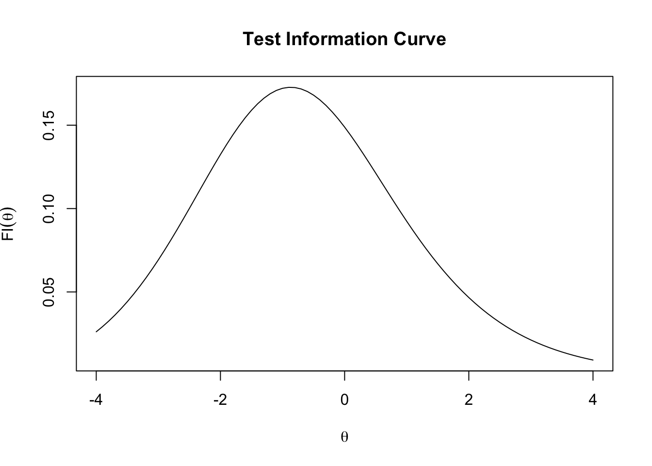
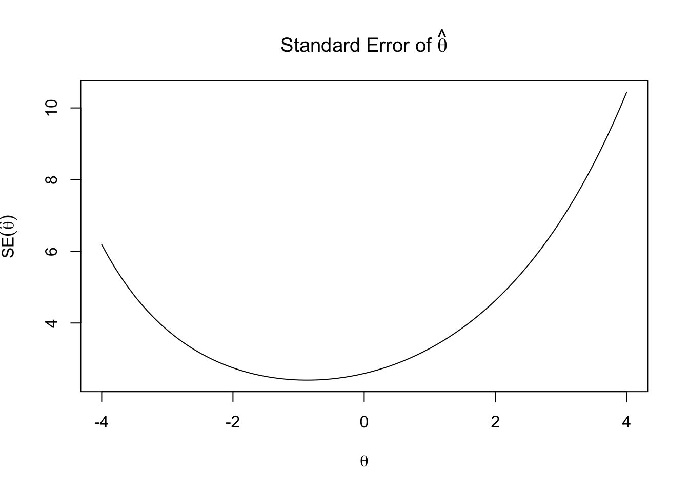
The standard error of \(\hat\theta\) is approximated by:
\[SE(\hat\theta) = \frac{1}{\sqrt{FI(\theta)}}\]
Let’s plot the standard error of ability estimate (\(SE(\hat\theta)\)).
SE <- 1 / sqrt(FI)
plot(theta_seq, SE,
     type="l",
     main = expression(paste("Standard Error of ", hat(theta))),
     ylab = expression(SE(hat(theta))),
     xlab=expression(theta))