Week 12 DIF Detection
In this chapter, we will illustrate several basic approaches to DIF screening. This includes:
Mantel-Haenszel DIF test (
difRpackage)Multiple-group IRT-based Test (
mirtpackage)Comparing ICCs
Here, we will use three data sets:
responses_difgrouptheta
The responses_dif is a dichotomous response matrix with 2000 rows (examinees) and 15 columns (items). The items are assumed to follow the 3PL model:
\[P_j(\theta) = c_j + \frac{1-c_j}{1+\exp[-D a_j(\theta - b_j)]}\]
responses_dif <- read.table("https://raw.githubusercontent.com/sunbeomk/PSYC490/main/respnoses_dif.txt")

dim(responses_dif)
## [1] 2000 15In addition to the responses, we also know the group membership of individuals. This is in the group vector:
group <- read.table("https://raw.githubusercontent.com/sunbeomk/PSYC490/main/group.txt")$x

length(group)
## [1] 2000## group
## F R
## 296 1704Here, F stands for the focal group, and R stands for the reference group. Note that this is a relatively unbalanced data set, where the focal group is a minority that only makes up about 15% of the sample. This is actually quite common in practice.
Another thing we note is that the true ability distribution of focal and reference group individuals can differ: We don’t observe true \(\theta\) in practice. However, for the current example, we simulated the responses based on individuals’ true thetas.
theta <- read.table("https://raw.githubusercontent.com/sunbeomk/PSYC490/main/theta.txt")$x

head(theta)
## [1] -0.13657947 -0.58848262
## [3] 0.04535149 -0.18486618
## [5] 0.84667377 1.64705571Just to illustrate the true \(\theta\) distribution in the two groups, let us do a boxplot.
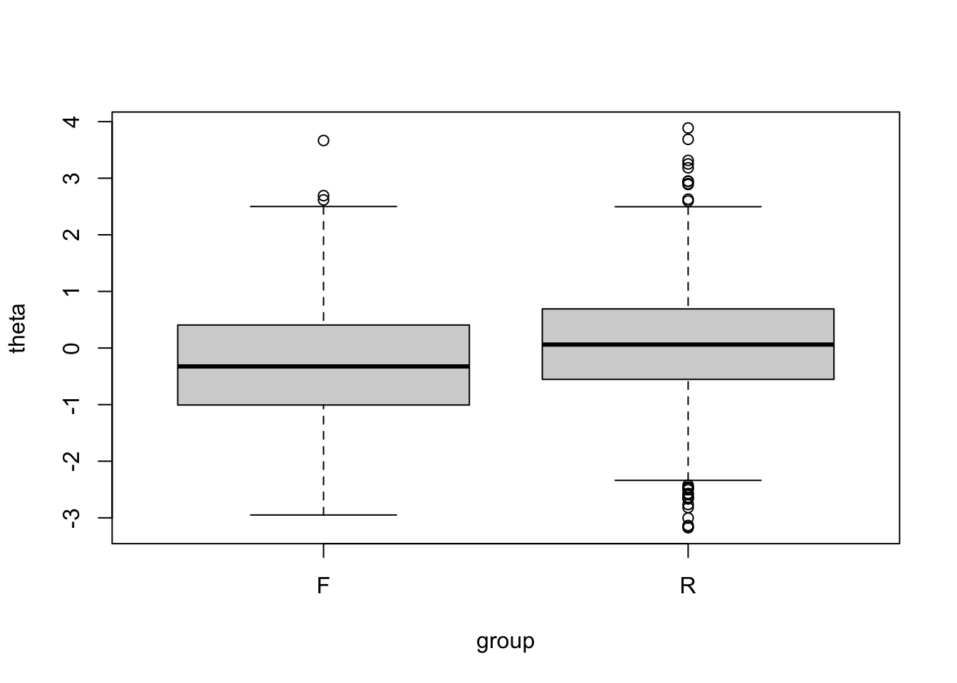
You can see that overall, the focal group individuals have higher proficiency. Therefore, if we observe group differences in the performance of an item, it could be due to impact (\(\theta\) difference) rather than bias (nuisance, construct-irrelevant factors). We only want to flag the latter in DIF screening.
Currently, we do not know which item has DIF. In the following, we will adopt the two methods (MH/Multiple-group IRT) and screen the 15 items one-by-one.
12.1 Mantel-Haenszel
To conduct the MH Test for DIF, we first need to install the difR package.
difR is an R package for a variety of DIF detection methods. For today, we will only use the Mantel-Haenszel Test functionality. If you want, you can explore this package by reading its pdf manual: https://cran.r-project.org/web/packages/difR/difR.pdf
We will use the difMH function for DIF screening w/ Mantel-Haenszel. Here are a few key arguments of the function (you can run ?difMH to read full documentation):
Data: The response data matrixgroup: Numeric or character. Vector of group membership.focal.name: The character/numeric label for the focal group. In our case, this isF(as in thegroupvector).purify: This is an optional argument By setting it to true, it performs “scale purification.”p.adjust.method: This is also an optional argument. Setting it to “BH” performs Benjamini-Hochberg adjustments to the p-values, to adjust for type-I error inflation due to multiple comparison.
Here is the command for implementing DIF detection using MH test for the responses_dif data:
out <- difMH(Data = responses_dif,
             group = group,
             focal.name = "F",
             purify = TRUE,
             p.adjust.method = "BH")
Let us adopt the categorization by ETS to label the 15 items:
A: \(H_0\) retained (\(p\geq.05\) using \(\alpha = .05\)) or effect size (\(|\Delta_{MH}|\leq 1\)). This means DIF is negligible, that is, there is no significant group difference, or the difference is very small.
C: \(H_0\) rejected (\(p<.05\)) and effect size \(|\Delta_{MH}|> 1.5\). This indicates an item has large DIF, meaning that group difference is statistically significant, and the difference is large in magnitude.
B: Everything between A and C. A weak indication of DIF.
At ETS, only C items are reviewed for bias by a DIF committee of trained test developers and subject experts.
##
## Detection of Differential Item Functioning using Mantel-Haenszel method
## with continuity correction and with item purification
##
## Results based on asymptotic inference
##
## Convergence reached after 2 iterations
##
## Matching variable: test score
##
## No set of anchor items was provided
##
## Multiple comparisons made with Benjamini-Hochberg adjustement of p-values
##
## Mantel-Haenszel Chi-square statistic:
##
##         Stat.   P-value
## item_1  31.4406  0.0000
## item_2   0.8849  0.3469
## item_3   3.1508  0.0759
## item_4   0.1431  0.7052
## item_5   0.3360  0.5621
## item_6   0.3665  0.5449
## item_7   1.3893  0.2385
## item_8   0.1650  0.6846
## item_9   1.0586  0.3035
## item_10  0.0047  0.9453
## item_11  6.4320  0.0112
## item_12  0.1140  0.7357
## item_13  1.6019  0.2056
## item_14  0.0088  0.9254
## item_15  0.3970  0.5286
##         Adj. P
## item_1   0.0000 ***
## item_2   0.7433
## item_3   0.3794
## item_4   0.8489
## item_5   0.8432
## item_6   0.8432
## item_7   0.7156
## item_8   0.8489
## item_9   0.7433
## item_10  0.9453
## item_11  0.0841 .
## item_12  0.8489
## item_13  0.7156
## item_14  0.9453
## item_15  0.8432
##
## Signif. codes: 0 '***' 0.001 '**' 0.01 '*' 0.05 '.' 0.1 ' ' 1
##
## Detection threshold: 3.8415 (significance level: 0.05)
##
## Items detected as DIF items:
##
##  item_1
##
##
## Effect size (ETS Delta scale):
##
## Effect size code:
##  'A': negligible effect
##  'B': moderate effect
##  'C': large effect
##
##         alphaMH deltaMH
## item_1   2.6304 -2.2728 C
## item_2   1.2663 -0.5548 A
## item_3   0.7454  0.6906 A
## item_4   0.9339  0.1607 A
## item_5   0.8971  0.2552 A
## item_6   1.1138 -0.2533 A
## item_7   1.2687 -0.5592 A
## item_8   0.9302  0.1701 A
## item_9   0.8372  0.4177 A
## item_10  0.9526  0.1140 A
## item_11  0.6160  1.1387 B
## item_12  1.0735 -0.1666 A
## item_13  1.2634 -0.5495 A
## item_14  1.0534 -0.1224 A
## item_15  1.3161 -0.6455 A
##
## Effect size codes: 0 'A' 1.0 'B' 1.5 'C'
##  (for absolute values of 'deltaMH')
##
## Output was not captured!
We can see that, item 1 was detected to have significant DIF (adjusted \(p<.001\)) with large effect size (\(|\Delta_{MH}|> 1.5\)). Therefore, item 1 belongs to category “C”. A negative \(\Delta_{MH}\) indicates that the item favors the reference group. Indeed, item 1 was the only item simulated to have DIF.
Let us see if the results from the Multiple-Group IRT method will agree.
12.2 Multiple-group IRT
To perform the multiple-group IRT DIF test, we need to first calibrate the item parameters for a question separately for focal and reference groups, and then determine whether the item parameters significantly differ across groups.
We will use the mirt package to perform likelihood ratio test to determine whether the first 5 items have DIF. To illustrate this, we use items 6 to 15 as the anchor set, i.e., items assumed to have no DIF.
The Multiple-group IRT method requires two steps:
Step 1: Fit a multiple group IRT model, using the
multipleGroupfunction inmirt. Here,invariancetells R which items are assumed to be DIF-free, in our cases, items 6:15, i.e.,colnames(responses_dif)[-(1:5)]Step 2: Perform hypothesis testing with the
DIFfunction. We feed in the results from the last step (dif_model).which.par =specifies the parameters to be compared across groups, anditems2testspecifies the set of items to perform hypothesis testing on.
##        groups converged
## item_1    F,R      TRUE
## item_2    F,R      TRUE
## item_3    F,R      TRUE
## item_4    F,R      TRUE
## item_5    F,R      TRUE
##            AIC   SABIC
## item_1 -30.703 -23.431
## item_2   0.354   7.626
## item_3   3.531  10.802
## item_4   5.694  12.966
## item_5   4.067  11.338
##             HQ     BIC     X2
## item_1 -24.533 -13.900 36.703
## item_2   6.524  17.157  5.646
## item_3   9.700  20.333  2.469
## item_4  11.864  22.497  0.306
## item_5  10.237  20.870  1.933
##        df     p adj_p
## item_1  3     0 0.000
## item_2  3  0.13 0.325
## item_3  3 0.481 0.733
## item_4  3 0.959 0.959
## item_5 3 0.586 0.733library(mirt)
dif_model <- multipleGroup(data = responses_dif,
model = 1,
itemtype = "3PL",
group = group,
invariance = c(colnames(responses_dif)[-c(1:5)], 'free_means', 'free_var'),
verbose = FALSE
)
dif_test <- DIF(MGmodel = dif_model,
which.par = c("a1", "d", "g"),
items2test = c(1:5),
p.adjust = "BH")
dif_testHere, by looking at the adjusted p-value, we can see that item 1 is detected with significant DIF again (\(p<.001\)).
12.3 Comparing ICCs
Plotting two ICCs for the reference and focal groups can visually aid in detecting DIF. Let’s draw ICCs of item 1 which had significant DIF in the previous analysis for the two groups.
From dif_model, we can extract the item parameter estimates for the two groups.
## $F
## $items
##             a      b     g u
## item_1  1.214  1.404 0.000 1
## item_2  2.249  1.425 0.000 1
## item_3  1.262  0.560 0.000 1
## item_4  1.342  0.292 0.097 1
## item_5  1.811  0.260 0.000 1
## item_6  1.102 -0.871 0.001 1
## item_7  1.843  0.931 0.000 1
## item_8  1.018  0.767 0.000 1
## item_9  1.314  0.464 0.000 1
## item_10 2.091  1.862 0.009 1
## item_11 1.312  1.797 0.000 1
## item_12 2.052  0.247 0.000 1
## item_13 1.418 -0.821 0.000 1
## item_14 1.601  1.903 0.007 1
## item_15 1.650  2.451 0.000 1
##
## $means
## F1
##  0
##
## $cov
##    F1
## F1  1
##
##
## $R
## $items
##             a      b     g u
## item_1  0.970  0.646 0.000 1
## item_2  1.496  1.663 0.012 1
## item_3  1.240  0.844 0.030 1
## item_4  1.087  0.109 0.000 1
## item_5  1.433  0.342 0.000 1
## item_6  1.102 -0.871 0.001 1
## item_7  1.843  0.931 0.000 1
## item_8  1.018  0.767 0.000 1
## item_9  1.314  0.464 0.000 1
## item_10 2.091  1.862 0.009 1
## item_11 1.312  1.797 0.000 1
## item_12 2.052  0.247 0.000 1
## item_13 1.418 -0.821 0.000 1
## item_14 1.601  1.903 0.007 1
## item_15 1.650  2.451 0.000 1
##
## $means
##    F1
## 0.375
##
## $cov
##       F1
## F1 0.979
Item parameter estimates for the focal and reference groups are:
# focal group
a_focal <- itempars_est[[1]]$items[, 1]
b_focal <- itempars_est[[1]]$items[, 2]
c_focal <- itempars_est[[1]]$items[, 3]
# reference group
a_ref <- itempars_est[[2]]$items[, 1]
b_ref <- itempars_est[[2]]$items[, 2]
c_ref <- itempars_est[[2]]$items[, 3]In order to draw ICC plots, we need irt.p function that computes the probability of correct response for a given \(\theta\) and item parameters. Note that mirt package uses IRF with the scale parameter \(D = 1\).
The next step is is to a sequence of \(\theta\) values.
Now, calculate the probability of correct response on item 1 for the focal and the reference groups corresponding to the sequence of \(\theta\) values.
p_item_f <- p_item_r <- numeric(length(theta_seq))

for (i in 1:length(theta_seq)) {
  p_item_f[i] <- irt_p(theta = theta_seq[i],
                       a = a_focal[1],
                       b = b_focal[1],
                       c = c_focal[1])
  p_item_r[i] <- irt_p(theta = theta_seq[i],
                       a = a_ref[1],
                       b = b_ref[1],
                       c = c_ref[1])
}
Below code chunk will draw two ICCs for the two groups.
lines()function overlays corresponding points to an existing plot.We can add a legend with
legend()function.
plot(theta_seq, p_item_f,
     type = "l", ylim=c(0, 1),
     xlab = expression(theta),
     ylab = expression(P(theta)),
     main = "ICC of Item 1",
     col = "red")

lines(theta_seq, p_item_r, col = "black")

legend("topleft",
       legend = c("focal", "reference"),
       col = c("red", "black"),
       lty = 1)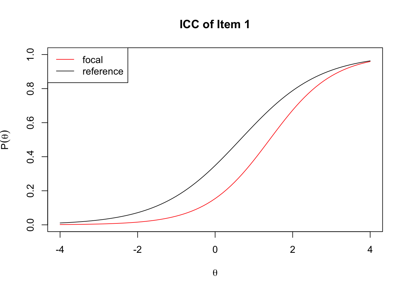
We can say that item 1 favors the reference group. Uniform DIF pattern is detected where the probability of correct response for the reference group is always greater than the focal group in the \(\theta\).