Week 13 IER
Examinees often display Insufficient Effort Responding (IER), especially in low-stakes tests. IER can be accounted for by lack of motivation or fatigue. Another factor contributing to IER is anonymity of online surveys/testings environment. Aberrant responses can reduce the reliability of the test, and consequently attenuate the validity of the test. Making decisions out of test scores that are unreliable and invalid may lead to undesirable results.
In this chapter, several methods for flagging IER will be demonstrated:
Long String
Psychometric Synonym/Antonym
Even-Odd Consistency
Mahalanobis Distance
These methods are implemented in the careless package. The example dataset used in this chapter is careless_dataset2 also contained in the careless package. Let’s import the careless package and save the careless_dataset2 dataset as data.
## [1] 1000 100The data is a simulated dataset with careless responses from 1,000 examinees on 100 items. It consists of 10 subscales.
##       [,1]     [,2]
##  [1,] "HSinc1" "HSinc2"
##  [2,] "HFair1" "HFair2"
##  [3,] "EAnxi1" "EAnxi2"
##  [4,] "EDepe1" "EDepe2"
##  [5,] "XLive1" "XLive2"
##  [6,] "AForg1" "AForg2"
##  [7,] "APati1" "APati2"
##  [8,] "CPerf1" "CPerf2"
##  [9,] "OInqu1" "OInqu2"
## [10,] "OUnco1" "OUnco2"
##       [,3]     [,4]
##  [1,] "HSinc3" "HSinc4"
##  [2,] "HFair3" "HFair4"
##  [3,] "EAnxi3" "EAnxi4"
##  [4,] "EDepe3" "EDepe4"
##  [5,] "XLive3" "XLive4"
##  [6,] "AForg3" "AForg4"
##  [7,] "APati3" "APati4"
##  [8,] "CPerf3" "CPerf4"
##  [9,] "OInqu3" "OInqu4"
## [10,] "OUnco3" "OUnco4"
##       [,5]     [,6]
##  [1,] "HSinc5" "HSinc6"
##  [2,] "HFair5" "HFair6"
##  [3,] "EAnxi5" "EAnxi6"
##  [4,] "EDepe5" "EDepe6"
##  [5,] "XLive5" "XLive6"
##  [6,] "AForg5" "AForg6"
##  [7,] "APati5" "APati6"
##  [8,] "CPerf5" "CPerf6"
##  [9,] "OInqu5" "OInqu6"
## [10,] "OUnco5" "OUnco6"
##       [,7]     [,8]
##  [1,] "HSinc7" "HSinc8"
##  [2,] "HFair7" "HFair8"
##  [3,] "EAnxi7" "EAnxi8"
##  [4,] "EDepe7" "EDepe8"
##  [5,] "XLive7" "XLive8"
##  [6,] "AForg7" "AForg8"
##  [7,] "APati7" "APati8"
##  [8,] "CPerf7" "CPerf8"
##  [9,] "OInqu7" "OInqu8"
## [10,] "OUnco7" "OUnco8"
##       [,9]     [,10]
##  [1,] "HSinc9" "HSinc10"
##  [2,] "HFair9" "HFair10"
##  [3,] "EAnxi9" "EAnxi10"
##  [4,] "EDepe9" "EDepe10"
##  [5,] "XLive9" "XLive10"
##  [6,] "AForg9" "AForg10"
##  [7,] "APati9" "APati10"
##  [8,] "CPerf9" "CPerf10"
##  [9,] "OInqu9" "OInqu10"
## [10,] "OUnco9" "OUnco10"
13.1 Long String
13.1.1 MaxLongString
The most straightforward way to detect IER is to find the length of the longest consecutive string (MaxLongString) of the same responses given by an examinee. For example, the 310th examinee answered all the items after item 21 identically. In this case, the MaxLongString is 79. A large enough MaxLongString may indicate IER.
##     HSinc1 HSinc2 HSinc3
## 310      3      3      5
##     HSinc4 HSinc5 HSinc6
## 310      3      2      5
##     HSinc7 HSinc8 HSinc9
## 310      6      5      3
##     HSinc10 HFair1 HFair2
## 310       7      4      3
##     HFair3 HFair4 HFair5
## 310      3      5      7
##     HFair6 HFair7 HFair8
## 310      7      1      2
##     HFair9 HFair10 EAnxi1
## 310      1       1      4
##     EAnxi2 EAnxi3 EAnxi4
## 310      6      6      6
##     EAnxi5 EAnxi6 EAnxi7
## 310      6      6      6
##     EAnxi8 EAnxi9 EAnxi10
## 310      6      6       6
##     EDepe1 EDepe2 EDepe3
## 310      6      6      6
##     EDepe4 EDepe5 EDepe6
## 310      6      6      6
##     EDepe7 EDepe8 EDepe9
## 310      6      6      6
##     EDepe10 XLive1 XLive2
## 310       6      6      6
##     XLive3 XLive4 XLive5
## 310      6      6      6
##     XLive6 XLive7 XLive8
## 310      6      6      6
##     XLive9 XLive10 AForg1
## 310      6       6      6
##     AForg2 AForg3 AForg4
## 310      6      6      6
##     AForg5 AForg6 AForg7
## 310      6      6      6
##     AForg8 AForg9 AForg10
## 310      6      6       6
##     APati1 APati2 APati3
## 310      6      6      6
##     APati4 APati5 APati6
## 310      6      6      6
##     APati7 APati8 APati9
## 310      6      6      6
##     APati10 CPerf1 CPerf2
## 310       6      6      6
##     CPerf3 CPerf4 CPerf5
## 310      6      6      6
##     CPerf6 CPerf7 CPerf8
## 310      6      6      6
##     CPerf9 CPerf10 OInqu1
## 310      6       6      6
##     OInqu2 OInqu3 OInqu4
## 310      6      6      6
##     OInqu5 OInqu6 OInqu7
## 310      6      6      6
##     OInqu8 OInqu9 OInqu10
## 310      6      6       6
##     OUnco1 OUnco2 OUnco3
## 310      6      6      6
##     OUnco4 OUnco5 OUnco6
## 310      6      6      6
##     OUnco7 OUnco8 OUnco9
## 310      6      6      6
##     OUnco10
## 310       6
The longstring() function in careless package calculates the MaxLongString for each examinee.
## [1] 79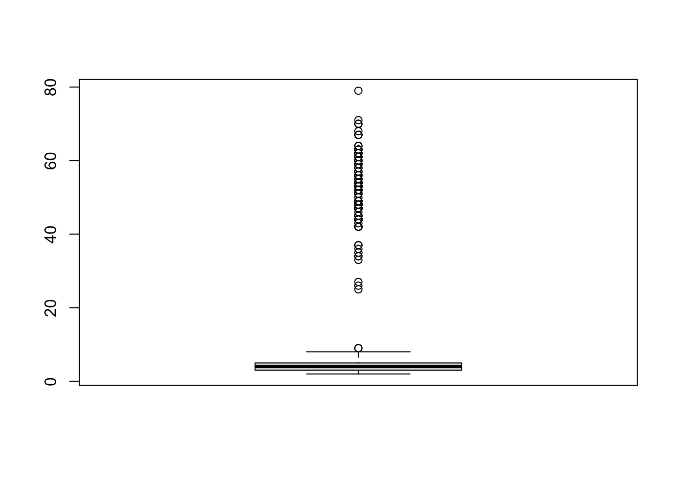
The boxplot of the the MaxLongString shows that some examinees may have responded a large proportion of consecutive items with insufficient effort. From the boxplot, we may decide to flag the examinees with MaxLongString greater than or equal to 20 to have IER.
##   [1]  14  17  36  39  64 107
##   [7] 120 125 126 157 160 165
##  [13] 181 189 198 200 223 225
##  [19] 227 232 236 239 249 256
##  [25] 269 272 282 296 297 309
##  [31] 310 318 328 332 335 342
##  [37] 354 362 377 386 391 398
##  [43] 417 419 423 429 438 455
##  [49] 469 471 473 480 483 506
##  [55] 529 542 544 556 558 561
##  [61] 571 572 591 604 607 624
##  [67] 625 639 649 663 672 682
##  [73] 683 698 699 701 712 722
##  [79] 726 728 732 736 740 745
##  [85] 759 767 783 788 803 805
##  [91] 809 823 825 843 856 857
##  [97] 863 873 881 886 904 905
## [103] 918 922 926 943 951 953
## [109] 979 981## [1] 110The number of detected IERs is 110.
13.1.2 AveLongStrong
Instead of calculating the length of the longest string of the same response, we can also see AveLongString which is the average length across all strings of the same response. For example, the AveLongString of the following response vector x can be calculated by:
## [1] 2 2 5 5 5 2 2 2 2 2\[\frac{2+3+5}{3} = 3.33\]
Again, the AveLongString index can be obtained by the longstring() function but with one additional argument.
## [1] 1.470588 1.351351 1.282051
## [4] 1.176471 1.315789 1.265823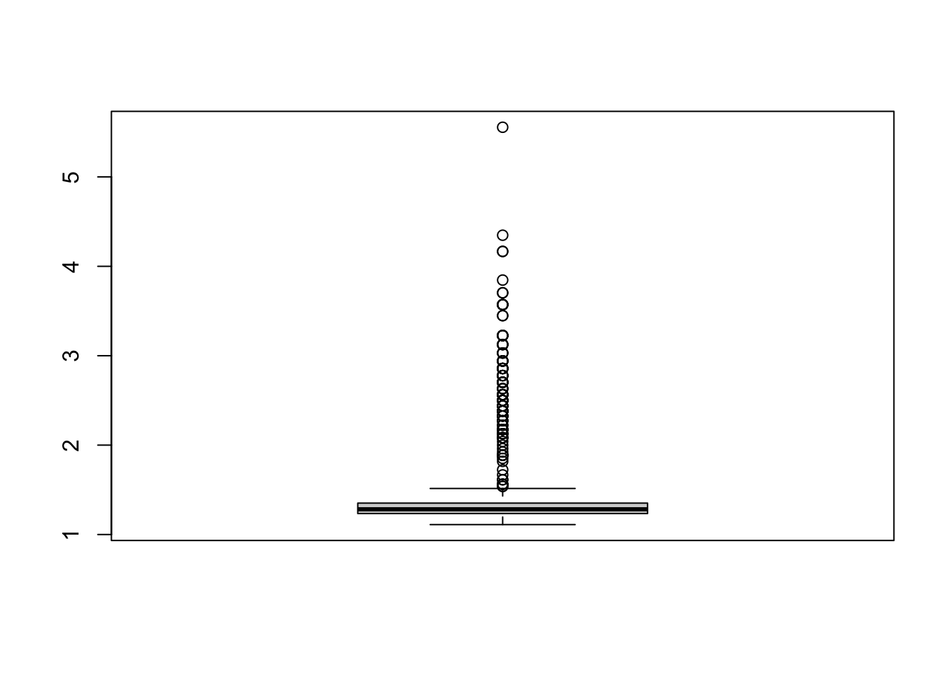
We can set the cut-off value as 2 and flag the examinees with AveLongString greater than or equal to 2 as IER.
##  [1]  17  36  39  64 120 125
##  [7] 126 157 160 165 181 198
## [13] 223 225 227 232 236 239
## [19] 249 256 269 272 282 296
## [25] 297 309 310 318 328 332
## [31] 335 342 354 362 377 386
## [37] 391 398 417 419 423 429
## [43] 438 455 469 471 473 480
## [49] 483 506 529 542 544 556
## [55] 558 561 572 591 604 607
## [61] 624 625 639 649 663 682
## [67] 698 701 712 722 726 728
## [73] 732 740 745 759 767 783
## [79] 788 803 809 823 825 843
## [85] 856 857 863 873 881 904
## [91] 905 918 922 926 943 951
## [97] 953 979 981## [1] 99The number of detected IERs is 99.
13.2 Psychometric Synonym/Antonym
The idea underlying psychometric synonym index is that pairs of items that bring out similar responses across the population should also do so for each individual. Similarly, psychometric antonym index implies that pairs of items that bring out opposite responses across the population should do so for each individual.
Flagging IER with psychometric synonym(antonym) involves two steps:
- Step 1: Calculate the pearson correlations between all possible pairs of items and then find the pairs of items with correlation greater than or equal to (less than or equal to) a cut-off value (e.g., .60).
##        Var1   Var2      Freq
## 6668 APati8 APati7 0.7893989
## 6567 APati7 APati6 0.7707801
## 6568 APati8 APati6 0.7365130
## 6669 APati9 APati7 0.7167873
## 7073 CPerf3 CPerf1 0.7106777- Step 2: Calculate the within-examinee correlation over these item pairs selected from Step 2. In other words, calculate the correlation between the set of 1st items from each pair and the set of 2nd items from each pair.
13.2.1 Step 1
The psychsyn_critval() function provides Step 1, and calculates the correlation between all pairs of items.
##        Var1   Var2      Freq
## 6668 APati8 APati7 0.7893989
## 6567 APati7 APati6 0.7707801
## 6568 APati8 APati6 0.7365130
## 6669 APati9 APati7 0.7167873
## 7073 CPerf3 CPerf1 0.7106777
## 6769 APati9 APati8 0.7049997## [1] 31The number of item pairs with correlation \(\geq .6\) is 31.
13.2.2 Step 2
The function psychsyn() calculates the psychometric synonyms index by setting the cut-off value as critval = .60.
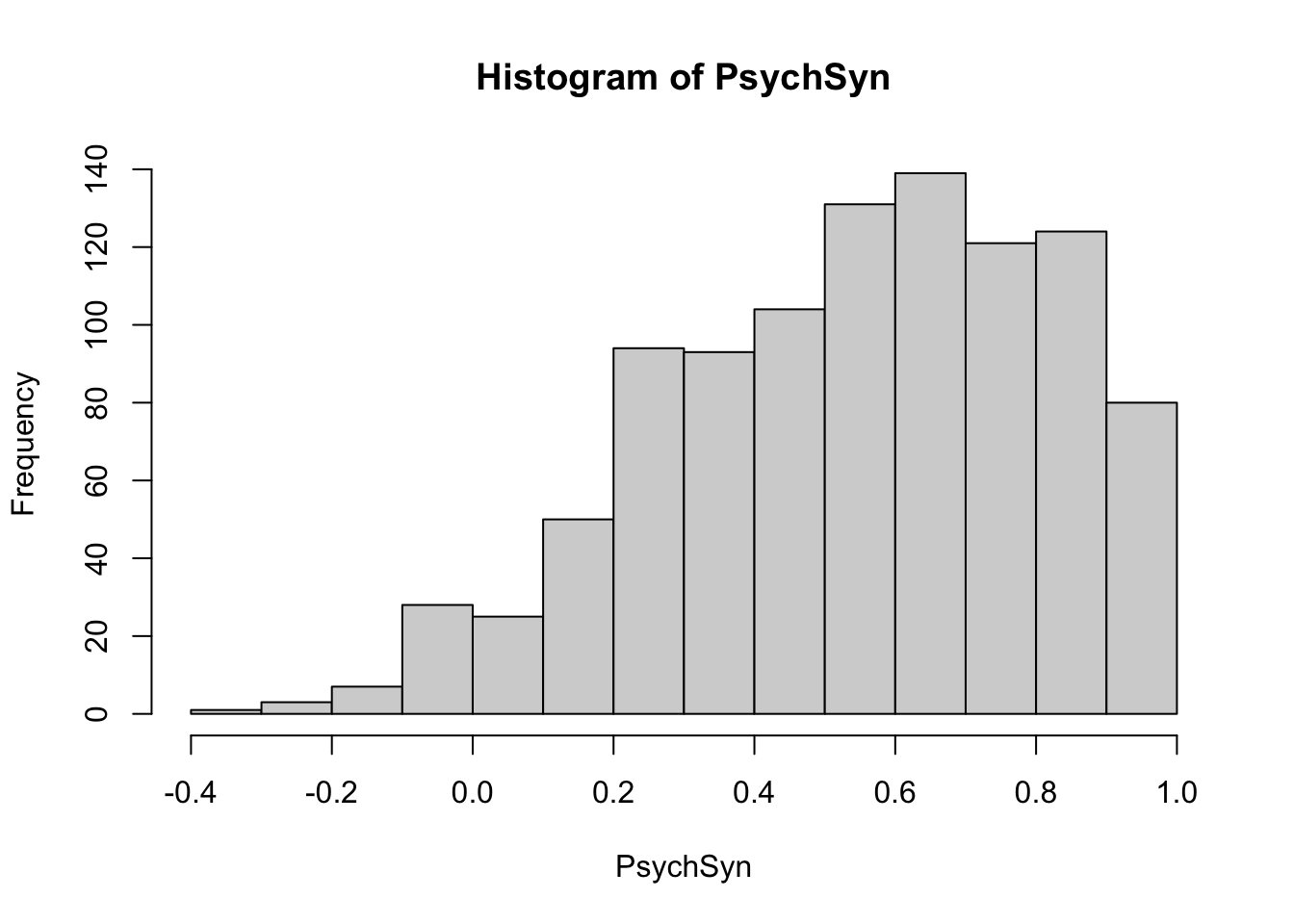
The psychometric synonym indices are centered around .60. Examinees whose correlations are close to zero or negative can be further inspected. Here, let’s find the examinees with psychometric synonym indices less than or equal to .20.
##   [1]   2  17  26  28  33  43
##   [7]  49  56  57  72  79  87
##  [13]  94 101 104 105 163 170
##  [19] 175 183 187 204 212 216
##  [25] 235 239 243 253 254 263
##  [31] 298 320 321 327 331 348
##  [37] 361 371 379 387 393 401
##  [43] 403 406 412 425 427 432
##  [49] 441 448 458 480 498 503
##  [55] 513 528 531 541 542 546
##  [61] 547 548 551 577 580 588
##  [67] 620 621 622 624 628 645
##  [73] 661 662 674 677 690 695
##  [79] 702 705 710 714 719 743
##  [85] 762 768 779 793 798 799
##  [91] 821 830 837 838 839 840
##  [97] 858 861 881 884 889 906
## [103] 910 916 921 932 933 938
## [109] 947 974 980 986 987 994## [1] 114The number of detected IERs is 114.
In order to obtain the psychometric antonym indices, use psychant() function instead of psychsyn() function. In this dataset, there are only two item pairs with correlations \(\leq -.60\). In this case, we may need to use another cut-off value or choose not to use psychometric antonym indices.
##        Var1   Var2       Freq
## 1018 HFair8 HFair1 -0.6290865
## 2126 EAnxi6 EAnxi2 -0.6242194
## 2226 EAnxi6 EAnxi3 -0.5951980
## 1318 HFair8 HFair4 -0.5882713
## 1017 HFair7 HFair1 -0.5852945
## 1317 HFair7 HFair4 -0.5683951## [1] 213.3 Even-Odd Consistency
Recall that the example dataset consists of 10 subscales. The even-odd consistency evaluates the correlation between scores on odd and even halves across subscales. For effortful examinees, the correlation between these two scores should be high. We can flag examinees with low even-odd consistency index as showing IER.
As an example, let’s calculates the even-odd consistency index of the first examinee. The below code chunk will obtain the sum score of even and odd items for each subscale.
# sum scores of even/odd items in each subscales
evenodd1 <- matrix(NA,
                   nrow=10, # number of subscales
                   ncol=2) # odd / even
colnames(evenodd1) <- c("odd_total","even_total")
rownames(evenodd1) <- paste0("subscale", 1:10)
for(i in 1:10){ # 10 subscales
  # odd_total
  evenodd1[i,1] <- sum(data[1, c(1,3,5,7,9) + 10*(i-1)])

  # even_total
  evenodd1[i,2] <- sum(data[1, c(2,4,6,8,10) + 10*(i-1)])
}
evenodd1
## odd_total
## subscale1 16
## subscale2 22
## subscale3 24
## subscale4 31
## subscale5 24
## subscale6 16
## subscale7 19
## subscale8 24
## subscale9 21
## subscale10 19
## even_total
## subscale1 11
## subscale2 18
## subscale3 20
## subscale4 31
## subscale5 19
## subscale6 20
## subscale7 15
## subscale8 28
## subscale9 28
## subscale10 18Now let’s calculate the correlation between the two scores. To correct for decreased length of the test, apply the Spearman-Brown formula to the split-half correlation .
\[r_{YY'} = \frac{N \times r_{XX'}}{1 + (N-1)r_{XX'}}\]
## [1] 0.8353962The even-odd consistency index of the first examinee is 0.8354.
The even-odd consistency indices of all examinees are obtained by using evenodd() function. The argument factors=rep(10,10) specifies the number of items in each subscale. Note that the evenodd() function returns the negative consistency indices (also called as inconsistency indices). Therefore, we multiply by -1 to obtain the consistency indices from the evenodd() function.
## Warning in evenodd(data, factors = rep(10, 10)): Computation of even-odd has changed for consistency of interpretation
##           with other indices. This change occurred in version 1.2.0. A higher
##           score now indicates a greater likelihood of careless responding. If
##           you have previously written code to cut score based on the output of
## this function, you should revise that code accordingly.## [1] 0.8353962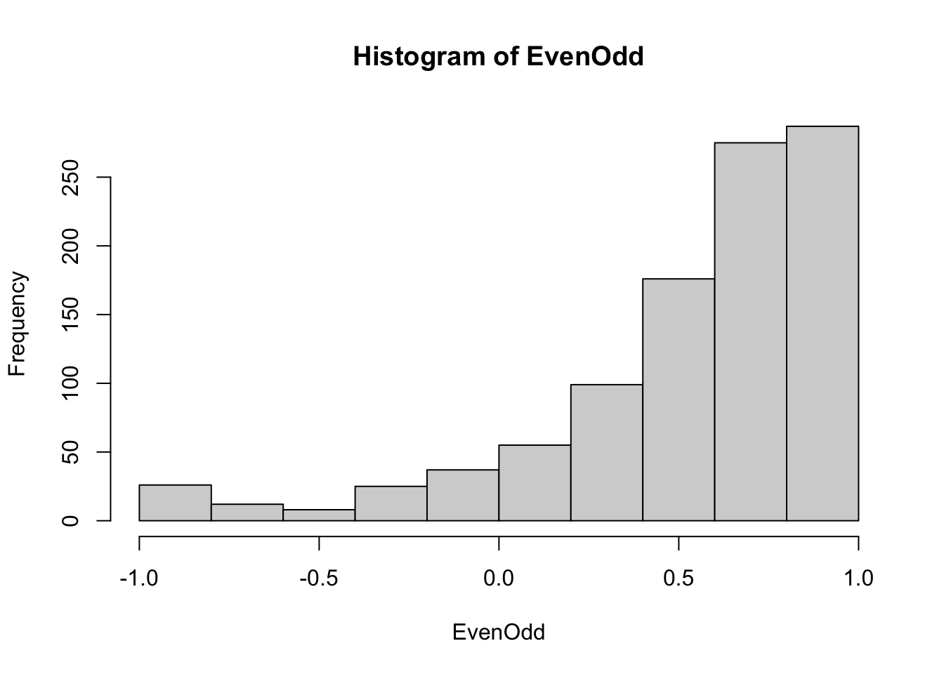
## [1] 107We can flag examinees with even-odd consistency index \(\leq 0\) as potential IERs. The number of flagged examinees is 107.
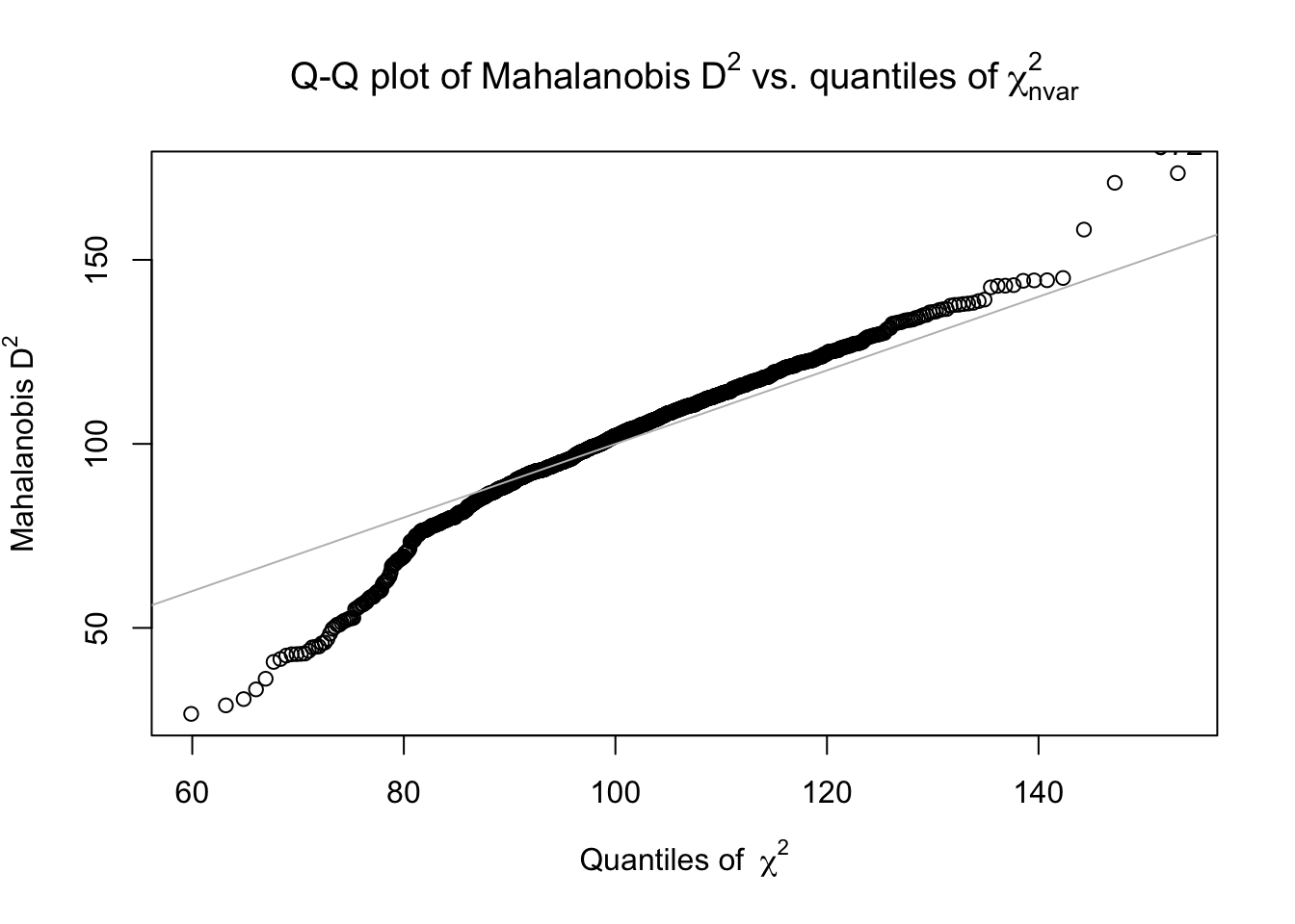
13.4 Mahalanobis Distance
The Mahalanobis Distance (MD) measures the squared distance between a person’s responses (\(x\)) to the center \(\bar{x}\). MD can be used to flag the multivariate outliers in the data. That is, we can flag examinees whose response vector is far from the distribution of all examinees. A large MD indicates a person doesn’t respond the same way as others.
The squared Mahalanobis Distance is obtained by:
\[(x-\bar{x})^T S^{-1} (x-\bar{x})\]
where \(S\) is the covariance matrix.
The below code chunk calculates the squared MD of the first examinee.
x <- as.matrix(data[1,]) # response vector of the first examinee

xbar <- colMeans(data) # vector of sample means

S <- cov(data) # covariance matrix

MD_1 <- (x-xbar) %*% solve(S) %*% t(x-xbar)
MD_1
## 1
## 1 99.1852The mahad() function calculates the squared MD for all examinee.
## [1] 99.1852## [1] 99.18520 85.90515
## [3] 79.46352 106.59060
## [5] 112.57374 95.04706If we assume that the items’ responses follow a multivariate normal distribution, the squared MD approximately follows a \(\chi^2_{df=n.items}\). We can flag the significantly large MD with one-sided \(p < .01\).
## [1] 135.8067## [1] 63 74 106 107 111 112
## [7] 115 135 285 346 416 588
## [13] 596 672 678 705 716 747
## [19] 846 852 866 889 916 933## [1] 24The number of flagged examinees are 24.
13.4.1 Flagged examinees
Let’s see how many flagged examinees overlap from each IER detection method.
LongStringFlag <- which(MaxLongString >= 20)

PsychSynFlag <- which(PsychSyn <= .20)

EvenOddFlag <- which(EvenOdd <= 0)

MDFlag <- which(MD > qchisq(.99, df=100))

Flag <- list(LongStringFlag, PsychSynFlag, EvenOddFlag, MDFlag)

Reduce(intersect, Flag)
## integer(0)No examinee was flagged in all four methods. The codes below will calculate the times each examinee was flagged and find the examinees who were flagged at least in two of the four methods.
NO.Flagged <- numeric(1000) # number of times that each examinee is flagged

for(i in 1:4){
  NO.Flagged[Flag[[i]]] <- NO.Flagged[Flag[[i]]] + 1
}

which(NO.Flagged >= 2)
## [1] 17 57 64 107 112 183
## [7] 187 189 239 298 416 480
## [13] 528 542 588 596 604 624
## [19] 645 661 672 705 821 881
## [25] 889 906 916 933 938References
Yentes R.D., & Wilhelm, F. (2021). careless: Procedures for computing indices of careless responding. R package version 1.2.1. (https://www.ryentes.com/careless/intro.html)