Week 6 Linear Regression

The objective of linear regression is to model a relationship between two sets of variables (e.g., \(X\) and \(Y\)). The result is a linear regression equation that can be used to make predictions — for example, if an examinee got a score of 5 on Test 1 (\(X\)), what is his/her expected criterion score on Test 2 (\(Y\))?

6.1 `cats` dataset from `MASS` package

An R package is a set of R functions, data, and documentations. There are over 18,000 packages available on the Comprehensive R Archive Network (CRAN) which is the public clearing house for R packages.

You can install an R package by install.packages("package_name")

We are going to use cats data as our toy example which is included in the MASS package. Let’s start with installing the MASS package.

install.packages("MASS")

You can find the list of installed packages on your library in the Packages tab of the View pane.

You can load and attach a package by:

library(MASS)

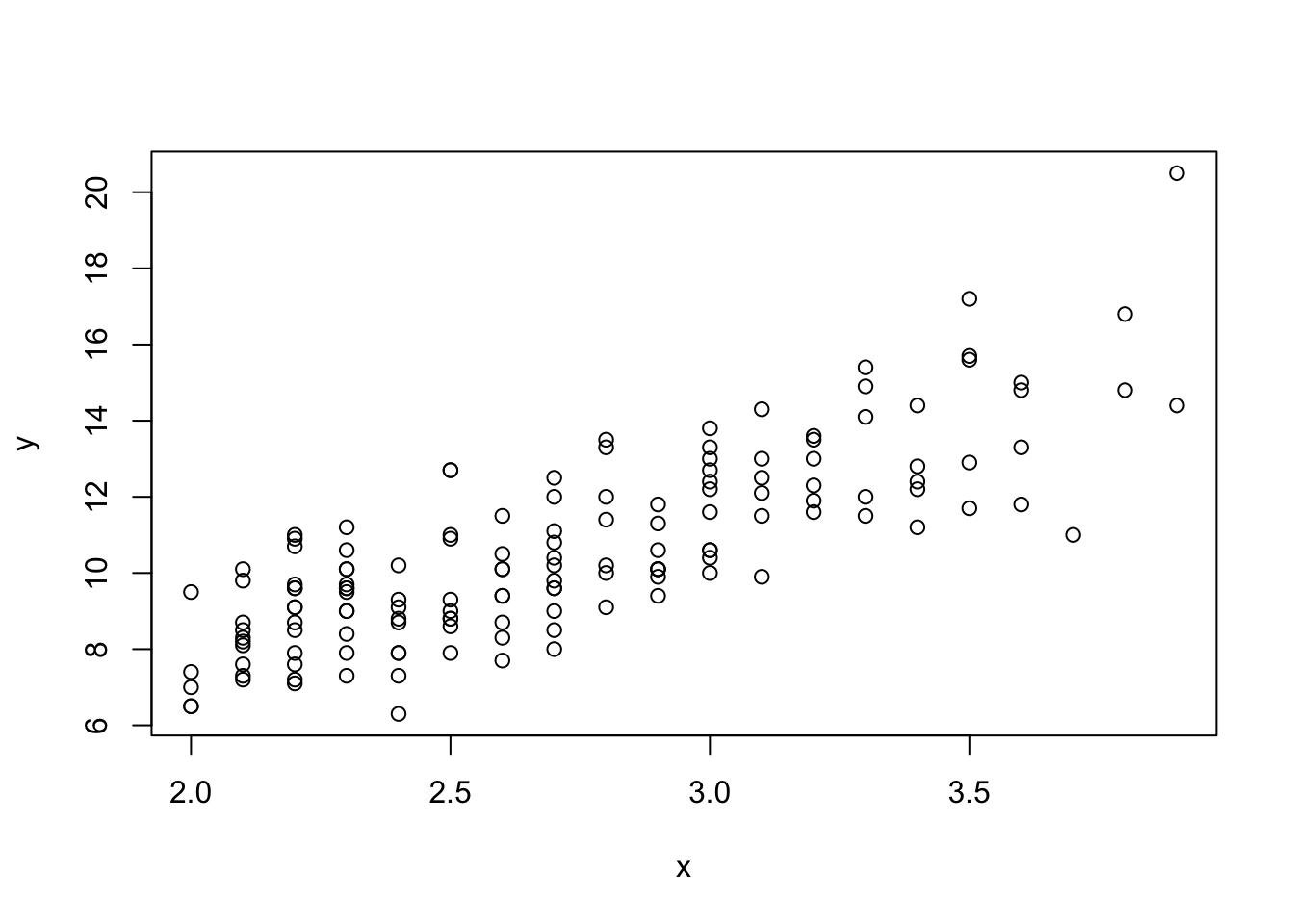
The cats data set included in the MASS package has three variables with 144 observations. The two numerical variables, Bwt and Hwt are the body weight and the heart weight of the cats.

data(cats)
dim(cats)

## [1] 144   3

head(cats)

##   Sex Bwt Hwt
## 1   F 2.0 7.0
## 2   F 2.0 7.4
## 3   F 2.0 9.5
## 4   F 2.1 7.2
## 5   F 2.1 7.3
## 6   F 2.1 7.6

Let’s use the last two variables (Bwt, Hwt) and save as x and y.

x <- cats$Bwt
y <- cats$Hwt

Scatter plots allow you to look at the relationship between two variables.

plot(x, y)

6.2 Simple Linear Regression

What regression tries to do is to find a straight line that best captures the linear relationship between the independent variable (IV, \(x\), predictor) and the dependent variable (DV, \(y\), predicted).

This straight line is found to minimize the residual sum of squares, that is, the sum of the squared distance between actual DV value and the corresponding point on the fitted line.

For such a line, there are two important coefficients:

Intercept (\(b_0\)): Value of DV when IV = 0;
Slope (\(b_1\)): Incremental change in DV when IV is increased by 1.

Then, we can characterize the regression line with the following equation: \[\hat y = b_0 + b_1 \cdot x\]

Here, \(\hat y\) is the predicted value of \(y\) (the corresponding point on the straight line).

We can obtain the numerical solutions for such a line:

\[\hat y = r_{xy}\frac{S_y}{S_x} (x - \bar x) + \bar y\]

\(r_{xy}\): Pearson correlation between IV (\(x\)) and DV (\(y\));
\(S_x\), \(S_y\): Sample standard deviations of \(x\) and of \(y\);
\(\bar x, \bar y\): Sample means.

If you do some algebraic manipulations, you’ll see that:

\(b_1 = r_{xy} \frac{S_y}{S_x};\)
\(b_0 = \bar y - \bar x \cdot r_{xy} \frac{S_y}{S_x}.\)

Let’s obtain the two regression coefficients, \(b_1\) and \(b_0\).

b1 <- cor(x, y) * (sd(y) / sd(x))
b0 <- mean(y) - mean(x) * b1
b1

## [1] 4.034063

b0

## [1] -0.3566624

You can use the regression coefficient values to predict \(y\) values from \(\hat y = b_1 \cdot x+b_0\). The predicted values \(\hat y\) are the predicted heart weight given the body weight.

yhat <- b1 * x + b0

The below plot shows the predicted heart weights values for corresponding body weights on the regression line.

plot(x, yhat)
points(mean(x), mean(y), col = "red", pch = 19)

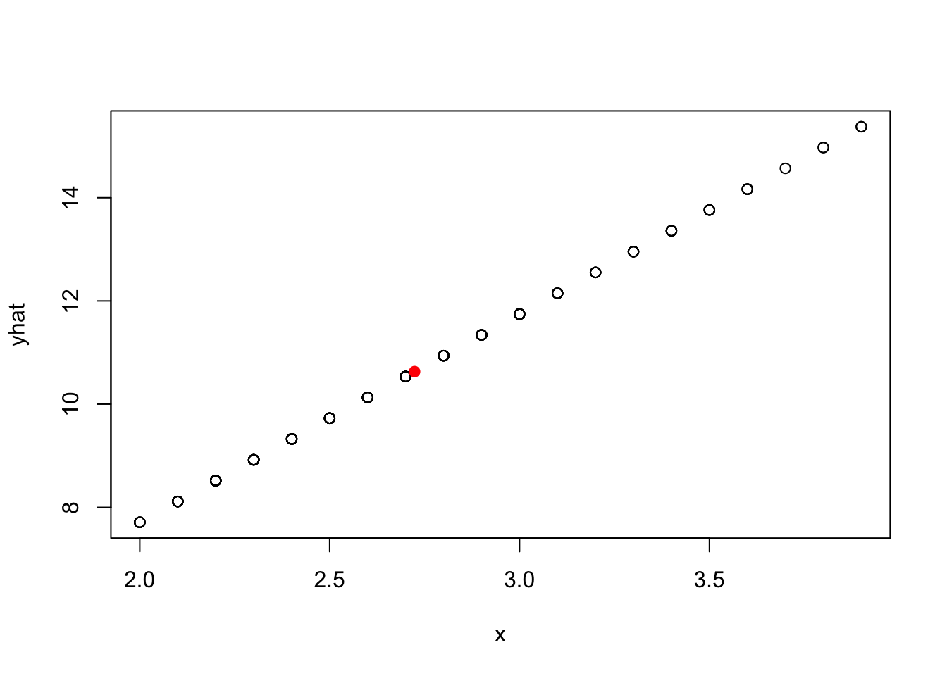
One of the important features of a simple linear regression line is that it always goes through \((\bar x, \bar y)\). The red dot in the above plot is \((\bar x, \bar y)\).

You can also predict the y value for specific x values. For example, if there are two new cats with body weights of 1.9 and 4.0, we can obtain the predicted heart weights, \(\hat y\) by:

new.x <- c(1.9, 4.0)
new.yhat <- b1 * new.x + b0
new.yhat

## [1]  7.308057 15.779588

The predicted heart weights of the new cats are 7.308 and 15.780.

plot(x, y, xlim = c(1, 5), ylim = c(6, 16))
abline(a = b0, b = b1)
points(mean(x), mean(y), col = "red", pch = 19)
points(new.x, new.yhat, col = "blue", pch = 19)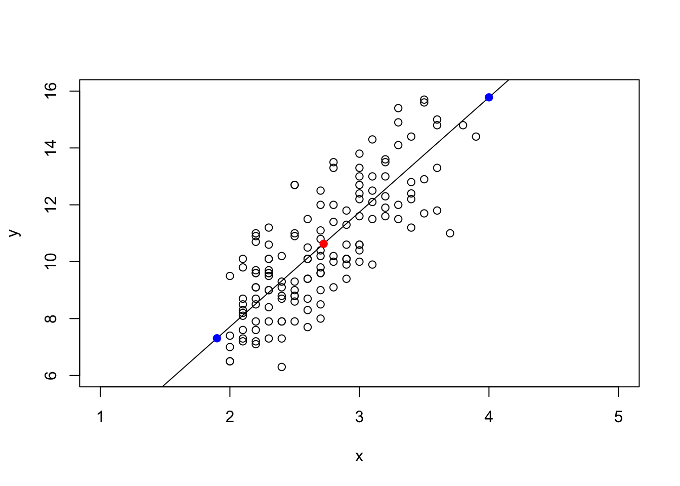

6.3 `lm()` function

Linear regression in R can be performed using the lm() function, standing for linear model.

For example, to predict the DV, y, from the IV, x, we can use lm(y ~ x).

Let’s fit a regression line to predict cat body weight based on cat heart weight.

Note, we give the lm() output a name, called cat_reg

cat_reg <- lm(y ~ x)

Or equivalently, you can fit exactly the same linear regression model by:

cat_reg2 <- lm(cats$Hwt ~ cats$Bwt)
cat_reg3 <- lm(Hwt ~ Bwt, data = cats)

The class of the output object is lm.

class(cat_reg)

## [1] "lm"

You can view the basic information of the regression output using the sumamry() function.

summary(cat_reg)

## 
## Call:
## lm(formula = y ~ x)
## 
## Residuals:
##     Min      1Q  Median 
## -3.5694 -0.9634 -0.0921 
##      3Q     Max 
##  1.0426  5.1238 
## 
## Coefficients:
##             Estimate
## (Intercept)  -0.3567
## x             4.0341
##             Std. Error
## (Intercept)     0.6923
## x               0.2503
##             t value Pr(>|t|)
## (Intercept)  -0.515    0.607
## x            16.119   <2e-16
##                
## (Intercept)    
## x           ***
## ---
## Signif. codes:  
##   0 '***' 0.001 '**' 0.01
##   '*' 0.05 '.' 0.1 ' ' 1
## 
## Residual standard error: 1.452 on 142 degrees of freedom
## Multiple R-squared:  0.6466, Adjusted R-squared:  0.6441 
## F-statistic: 259.8 on 1 and 142 DF,  p-value: < 2.2e-16

You can extract the vector of regression coefficients from an lm class object.

cat_reg$coefficients

## (Intercept)           x 
##  -0.3566624   4.0340627

Let’s compare the regression coefficients with b0 and b1 we calculated without the lm() function.

cat_reg$coefficients

## (Intercept)           x 
##  -0.3566624   4.0340627

b0

## [1] -0.3566624

b1

## [1] 4.034063

If you want to predict the DV (\(y\)) given a value of the IV (\(x\)), you can use the predict() function in R. In fact, you can also get the confidence intervals for the prediction.

predict(cat_reg, data.frame(x = c(1.9, 4.0)), 
        interval = "confidence",
        level = .95)

##         fit       lwr
## 1  7.308057  6.835548
## 2 15.779588 15.104327
##         upr
## 1  7.780565
## 2 16.454850

Week 6 Linear Regression

6.1 cats dataset from MASS package

6.2 Simple Linear Regression

6.3 lm() function

6.1 `cats` dataset from `MASS` package

6.3 `lm()` function