Week 10 Item Response Theory 1

Item response theory models the nonlinear relationship between the examinee’s trait level $\theta_i$ and the response probability $P_j(\theta_i)$ on the items. A few item response functions that are commonly used are:

1PL: $P_j(\theta_i) =\frac{1}{1+\exp[-Da(\theta_i - b_j)]}$
2PL: $P_j(\theta_i) = \frac{1}{1+\exp[-Da_j(\theta_i - b_j)]}$
3PL: $P_j(\theta_i) = {c_j} + \frac{{1-c_j}}{1+\exp[-Da_j(\theta_i - b_j)]}$

Here:

$P_j(\theta_i) = P(Y_{ij}=1\mid \theta_i)$ provides the probability of correct response on item $j$ , given ability $\theta_i$ .
$Y_{ij}=0/1$ is the response to question $j$ by examinee $i$
$\theta_i$ is the latent trait value (e.g., ability) of examinee $i$
$b_j:$ Difficulty (ability required by item)
$a_j:$ Discrimination (change rate of correct probability as a function of $(\theta_i - b_j)$ )
$c_j:$ Pseudoguessing parameter. Chance of correct response for someone with infinitely low ability.
$D$ : Some scaling constant, usually set to $1.7$ or $1$ .

In addition, one common way of fixing the scale of IRT models is:

Standardize $\theta$ so that $\mu = 0$ and $\sigma = 1$ .
So, $\theta$ is commonly (not always) assumed to follow the standard normal distribution ( $N(0,1)$ ).
Although $N(0,1)$ random variables can range between $-\infty$ and $\infty$ , most of the data ( $>99\%$ ) will be between $-4$ and $4$ .

In this chapter, students will learn how to plot item characteristic curves and to generate random responses data under item response theory models.

10.1 Item Characteristic Curves (ICC)

10.1.1 Item parameters

The following data set GRE40 contains the item parameters of 40 items following the 3PL model. Therefore, each item has $a_j, b_j, c_j$ parameters.

GRE40 <- read.table("https://raw.githubusercontent.com/sunbeomk/PSYC490/main/GRE40.txt")
head(GRE40)

##   item_ID    a     b    c
## 1       1 0.26 -1.30 0.04
## 2       2 0.40  1.00 0.15
## 3       3 0.43 -2.00 0.14
## 4       4 0.49 -0.60 0.00
## 5       5 0.52 -1.55 0.12
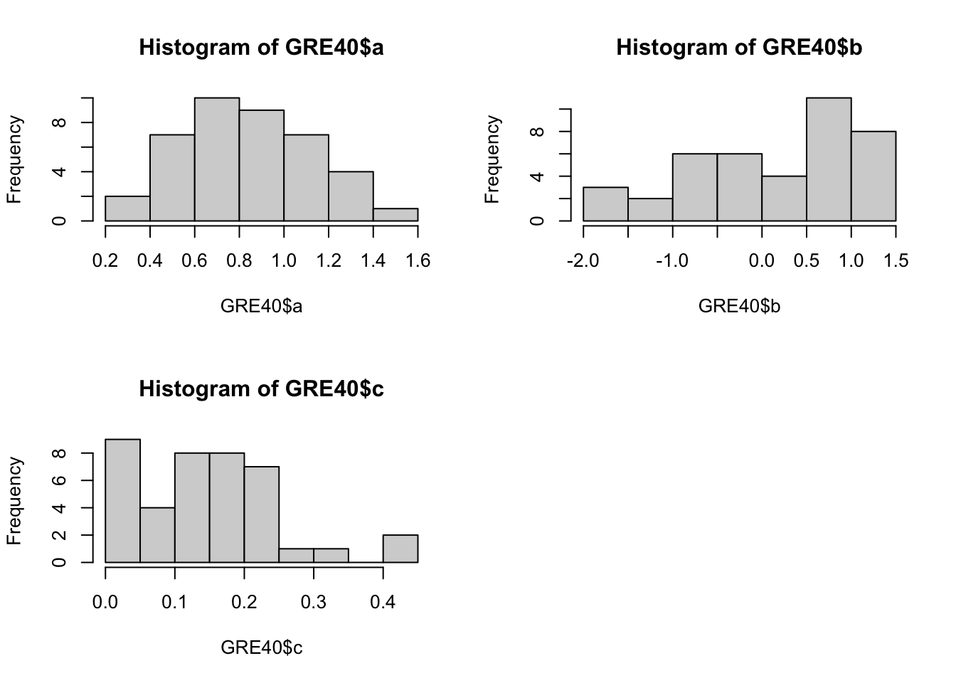
## 6       6 0.55  0.71 0.00

Let’s first see what these parameter values look like.

hist(GRE40$a)

hist(GRE40$b)

hist(GRE40$c)

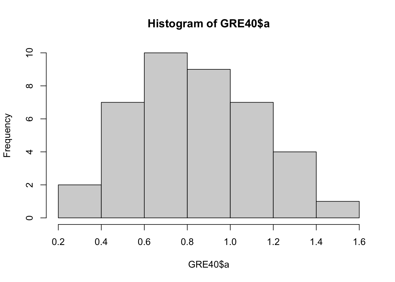
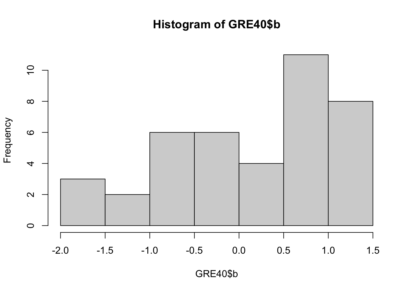
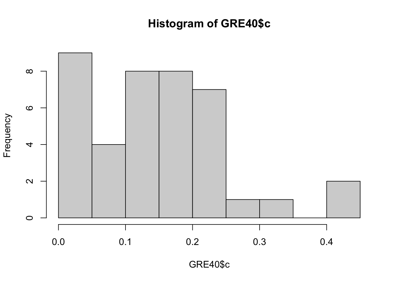
You can draw multiple plots in a single window by setting the graphical parameters in par() function. Below code will set the graphical parameters such that the subsequent plots are drawn in an 1-by-3 array by rows. That is, we can plot three histograms in a single window.

par(mfrow=c(1,3))
hist(GRE40$a)
hist(GRE40$b)
hist(GRE40$c)

par(mfrow=c(1,1))

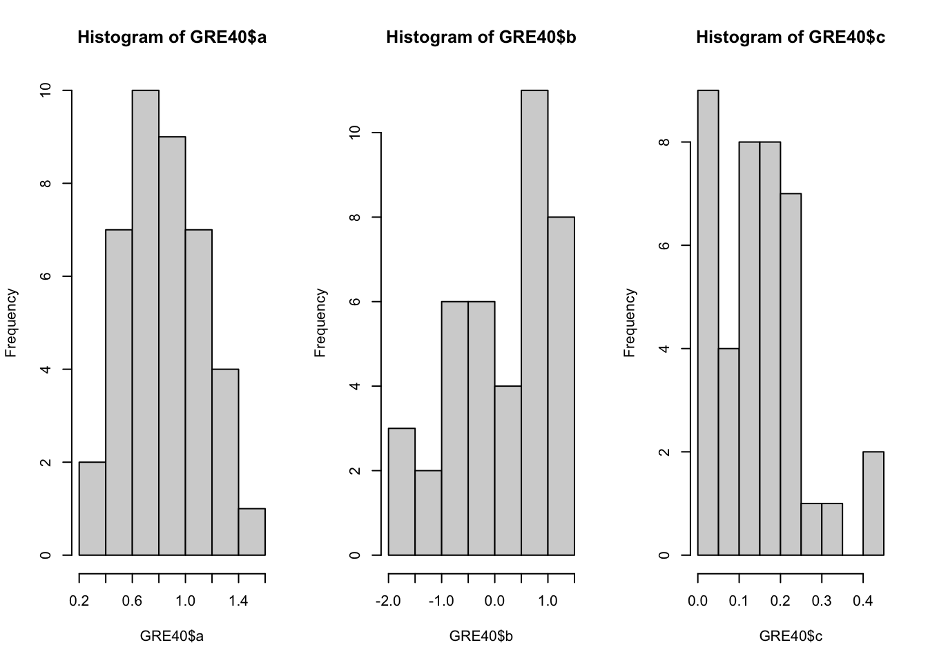
Below code chunk will draw the three histograms in a 2-by-2 array, by row.

par(mfrow=c(2,2))
hist(GRE40$a)
hist(GRE40$b)
hist(GRE40$c)
par(mfrow=c(1,1))

10.1.2 Drawing ICC plots

One important way of visualizing IRT models is to draw item characteristic curves (ICC curves). The ICC curve is essentially a curve for an item $j$ that plots the relationship between

$\theta$ : ability of examinee; and
$P_j(\theta)$ : probability of answering $j$ correctly.

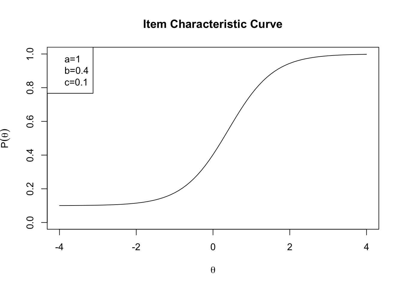
As ability changes, probability of correct response also changes. The ICC shows how it changes. What we want to do next is to draw ICCs for each GRE40 item. Plotting an ICC involves a few steps.

Step 1: Create a function for the IRF
Step 2: Create a sequence of theta values
Step 3: Evaluate $P_j$ at a series of $\theta$ s
Step 4: Plot $P_j$ vs $\theta$ as a curve.

10.1.2.1 Step 1: Create a function for the IRF

We need to compute $P_j(\theta)$ for a given $\theta$ value. We will create an R function that calculates $P_j(\theta) = P(correct)$ , when $\theta$ is the input. The function below, irt_p(), can be used to calculate $P_j(\theta)$ for a 3PL item, given specific $a, b, c$ parameter values. Here, we assume $D = 1.7$ .

irt_p <- function(theta, a, b, c){   #ability and item parameters as scalars
  p <- c + (1 - c) / (1 + exp(-1.7 * a * (theta - b)))
  
  p
}

Take a look at the function:

What are its inputs?
What does p calculate?
What is the output?

In sum, this function is created, so that it returns $P_j(Y_{ij}=1\mid \theta_i,a_j, b_j, c_j)$ by evaluating these values in the 3PL formula: $P_j(\theta_i) = {c_j} + \frac{{1-c_j}}{1+\exp[-Da_j(\theta_i - b_j)]}$ Let’s now try to plug in a few values.

irt_p(theta = 0, a = 1, b = -.2, c = .25)

## [1] 0.6881429

irt_p(theta = -1, a = 1, b = -.2, c = .25)

## [1] 0.4031802

10.1.2.2 Step 2: Create a sequence of theta values

Drawing an ICC curve involves finding finding $P_j(\theta)$ for a variety of $\theta$ values. In other words:

We want to look at a variety of possible $\theta$ values: $\theta = -4, -3.9, \ldots, -.1, 0, .1, \ldots, 3.9, 4$ .
For each of these $\theta$ values, we calculate $P_j(\theta)$ .
Then we can plot these two in a curve.

We can use the seq() function to create a vector of equally spaced numbers. Specifically, seq(from = m, to = n, by = d) creates a sequence, where it starts from $m$ , ends at $n$ , and each time increases by $d$ . The code chunk below creates a $\theta$ sequence that starts at $-4$ , ends at $4$ , and each time increases by $.1$ .

theta_seq <- seq(from = -4, to = 4, by = .1)
theta_seq

##  [1] -4.0 -3.9 -3.8 -3.7 -3.6
##  [6] -3.5 -3.4 -3.3 -3.2 -3.1
## [11] -3.0 -2.9 -2.8 -2.7 -2.6
## [16] -2.5 -2.4 -2.3 -2.2 -2.1
## [21] -2.0 -1.9 -1.8 -1.7 -1.6
## [26] -1.5 -1.4 -1.3 -1.2 -1.1
## [31] -1.0 -0.9 -0.8 -0.7 -0.6
## [36] -0.5 -0.4 -0.3 -0.2 -0.1
## [41]  0.0  0.1  0.2  0.3  0.4
## [46]  0.5  0.6  0.7  0.8  0.9
## [51]  1.0  1.1  1.2  1.3  1.4
## [56]  1.5  1.6  1.7  1.8  1.9
## [61]  2.0  2.1  2.2  2.3  2.4
## [66]  2.5  2.6  2.7  2.8  2.9
## [71]  3.0  3.1  3.2  3.3  3.4
## [76]  3.5  3.6  3.7  3.8  3.9
## [81]  4.0

10.1.2.3 Step 3: Evaluate $P_j$ at a series of $\theta$ s

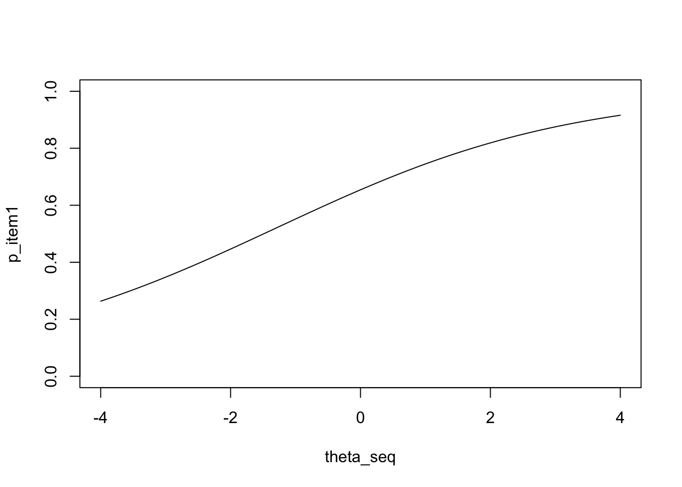
Our next step would be calculating $P_j(\theta_i)$ at each of these $\theta$ s between $-4$ and $4$ . We’ll illustrate this with item $1$ . Let’s create a for loop to calculate $P_j(\theta_i)$ for each $\theta_i \in [-4,4]$ .

p_item1 <- numeric(length(theta_seq))
for (t in 1:length(theta_seq)) {
  p_item1[t] <- irt_p(theta = theta_seq[t],
                   a = GRE40$a[1],
                   b = GRE40$b[1],
                   c = GRE40$c[1])
}

Notice that the question takes $t$ th $\theta$ (theta_seq[t]) and item 1’s parameters as input, and outputs the corresponding $P_j$ .

10.1.2.4 Step 4: Plot $P_j$ vs $\theta$ as a curve.

Now we have the $x$ axis ( $\theta$ ) and the $y$ axis ( $P_j$ ), we can draw the ICC curve.

plot(theta_seq, p_item1, 
     type = 'l', 
     ylim = c(0, 1))

Note that type = 'l' tells R that you want to connect the points on the plot with a line (curve).

10.2 Simulating Data Under IRT Models

What we have above define a data generating model. In other words, as long as we have all these information:

True $\theta$ distribution
Item response model
Item parameters

We can randomly generate data under an IRT model. That is, we can create a hypothetical data set. This can be convenient for many tasks such as conducting simulation studies. Here, we will generate $1000$ subjects’ responses on $40$ GRE items. Generating random responses involves several steps.

Step 1: Randomly generate ability $\theta$ s from the standard normal distribution
Step 2: Calculate $P_j(\theta_i)$ using the item response function
Step 3: Randomly generate $Y_{ij}$ from Bernoulli( $p_{ij}$ )

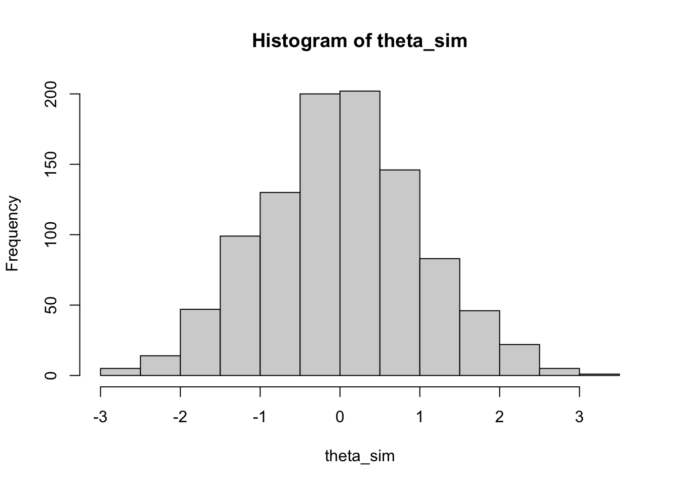
10.2.0.1 Step 1: Randomly generate $\theta$ s

Because we assumed the true abilities $\theta \sim N(0,1)$ , we can use rnorm to randomly generate some standard normal variables. These will be $1000$ hypothetical examinees’ true abilties.

set.seed(123)
theta_sim <- rnorm(1000)
hist(theta_sim)

10.2.0.2 Step 2: Calculate $P_j(\theta_i)$

To simulate $Y_{ij}$ s, we need to know each examinees’ correct response probability to each item. Let us create a for loop that calculates:

P(correct) for each of the 40 items; for
all 1000 examinees.

n_subjects <- 1000
n_items <- 40
pij <- matrix(NA, n_subjects, n_items) # 1000-by-40 matrix
for (i in 1:n_subjects) {
    for (j in 1:n_items) {
      pij[i, j] <- irt_p(theta_sim[i], GRE40$a[j], GRE40$b[j], GRE40$c[j])
    }
}

The outcome vector pij is a 1000 by 40 matrix, where the $(i, j)$ element is the probability of correct response for examinee $i$ on item $j$ .

10.2.0.3 Step 3: Randomly generate $Y_{ij}$ from Bernoulli( $p_{ij}$ )

One way to do this is using rbinom. For example, for $1$ st examinee on $1$ st item:

i <- 1
j <- 1
Y_ij <- rbinom(1, 1, prob = pij[i, j])
Y_ij

## [1] 1

Let’s use a for loop to generate the response matrix.

resp <- matrix(NA, n_subjects, n_items)
for (i in 1:n_subjects) {
  for (j in 1:n_items) {
    resp[i, j] <- rbinom(1, 1, prob = pij[i, j])
  }
}
head(resp)

##      [,1] [,2] [,3] [,4] [,5]
## [1,]    1    0    1    1    1
## [2,]    1    0    1    0    0
## [3,]    1    0    1    1    1
## [4,]    0    0    1    0    1
## [5,]    1    1    1    1    0
## [6,]    1    0    1    1    1
##      [,6] [,7] [,8] [,9]
## [1,]    0    0    0    0
## [2,]    1    0    0    0
## [3,]    1    0    0    1
## [4,]    1    1    0    1
## [5,]    0    1    1    0
## [6,]    1    1    1    1
##      [,10] [,11] [,12] [,13]
## [1,]     0     1     1     1
## [2,]     1     1     0     1
## [3,]     1     1     1     1
## [4,]     1     1     1     1
## [5,]     1     1     1     1
## [6,]     1     1     1     1
##      [,14] [,15] [,16] [,17]
## [1,]     0     1     1     1
## [2,]     0     1     0     0
## [3,]     1     1     0     1
## [4,]     1     1     1     0
## [5,]     0     1     1     0
## [6,]     1     1     1     1
##      [,18] [,19] [,20] [,21]
## [1,]     0     1     1     0
## [2,]     1     0     0     0
## [3,]     1     1     1     1
## [4,]     1     1     1     1
## [5,]     0     0     1     0
## [6,]     1     1     1     1
##      [,22] [,23] [,24] [,25]
## [1,]     0     0     0     0
## [2,]     1     0     0     1
## [3,]     1     0     1     1
## [4,]     1     0     0     1
## [5,]     1     0     1     1
## [6,]     1     1     0     1
##      [,26] [,27] [,28] [,29]
## [1,]     0     0     1     0
## [2,]     0     0     0     1
## [3,]     1     1     1     1
## [4,]     0     0     1     1
## [5,]     1     1     1     1
## [6,]     1     1     1     1
##      [,30] [,31] [,32] [,33]
## [1,]     0     0     0     0
## [2,]     0     1     0     0
## [3,]     1     1     1     1
## [4,]     0     1     1     1
## [5,]     1     0     1     0
## [6,]     1     1     1     1
##      [,34] [,35] [,36] [,37]
## [1,]     0     1     0     0
## [2,]     0     1     0     1
## [3,]     1     1     0     1
## [4,]     0     1     0     0
## [5,]     1     0     1     1
## [6,]     1     1     0     1
##      [,38] [,39] [,40]
## [1,]     1     0     0
## [2,]     1     0     0
## [3,]     1     0     0
## [4,]     0     0     1
## [5,]     0     0     1
## [6,]     1     0     1

Now, resp is the response matrix we created. In practice, after administering the test, the only thing we get might be resp. That is, we do not know the true $\theta$ s (theta_sim). In the next chapter, we will use this resp data set to plot empirical ICCs and to estimate individuals’ $\theta$ s.