4.3 The JM package
Now it is time to fit these models in R. To this end, we need first to fit separately the linear mixed effect model and the Cox model, and then take the returned objects and use them as main arguments in the jointModel function. The dataset used is the same that the one seen with the mixed model, aids. The survival information can be found in aids.id.
head(aids)
##   patient  Time death       CD4 obstime drug gender prevOI         AZT
## 1       1 16.97     0 10.677078       0  ddC   male   AIDS intolerance
## 2       1 16.97     0  8.426150       6  ddC   male   AIDS intolerance
## 3       1 16.97     0  9.433981      12  ddC   male   AIDS intolerance
## 4       2 19.00     0  6.324555       0  ddI   male noAIDS intolerance
## 5       2 19.00     0  8.124038       6  ddI   male noAIDS intolerance
## 6       2 19.00     0  4.582576      12  ddI   male noAIDS intolerance
##   start  stop event
## 1     0  6.00     0
## 2     6 12.00     0
## 3    12 16.97     0
## 4     0  6.00     0
## 5     6 12.00     0
## 6    12 18.00     0

head(aids.id)
##   patient  Time death       CD4 obstime drug gender prevOI         AZT
## 1       1 16.97     0 10.677078       0  ddC   male   AIDS intolerance
## 2       2 19.00     0  6.324555       0  ddI   male noAIDS intolerance
## 3       3 18.53     1  3.464102       0  ddI female   AIDS intolerance
## 4       4 12.70     0  3.872983       0  ddC   male   AIDS     failure
## 5       5 15.13     0  7.280110       0  ddI   male   AIDS     failure
## 6       6  1.90     1  4.582576       0  ddC female   AIDS     failure
##   start stop event
## 1     0  6.0     0
## 2     0  6.0     0
## 3     0  2.0     0
## 4     0  2.0     0
## 5     0  2.0     0
## 6     0  1.9     1
The idea here is to test for a treatment effect on survival after adjusting for the CD4 cell count.6
lattice::xyplot(sqrt(CD4) ~ obstime | drug, group = patient, data = aids,
    xlab = "Months", ylab = expression(sqrt("CD4")), col = 1, type = "l")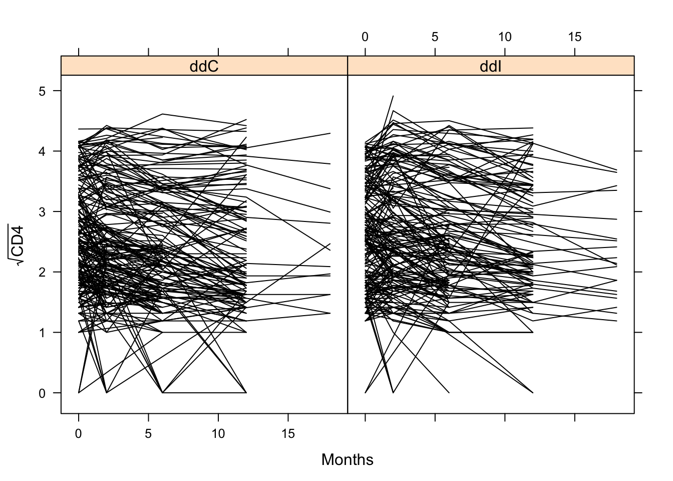
lattice::xyplot(sqrt(CD4) ~ obstime | patient, group = patient,
       data = aids[aids$patient %in% c(1:10),],
       xlab = "Months", ylab = expression(sqrt("CD4")), col = 1, type = "b")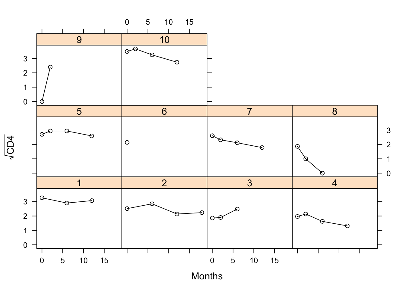
Now we are going to specify and fit a joint model. The linear mixed effects model for the CD4 cell counts include:
- Fixed-effects part: main effect of time and the interaction with the treatment.
- random-effects design matrix: an intercept and a time term.
The survival submodel include: treatment effect (as a time-independent covariate) and the true underlying effect of CD4 cell count as estimated from the longitudinal model (as time-dependent). The baseline risk function is assumed piecewise constant.
fitLME <- lme(sqrt(CD4) ~ obstime : drug, random = ~ obstime | patient, data = aids)
fitSURV <- coxph(Surv(Time, death) ~ drug, data = aids.id, x = TRUE)
fitJM <- jointModel(fitLME, fitSURV, timeVar = "obstime", method = "piecewise-PH-GH")
summary(fitJM)
##
## Call:
## jointModel(lmeObject = fitLME, survObject = fitSURV, timeVar = "obstime",
##     method = "piecewise-PH-GH")
##
## Data Descriptives:
## Longitudinal Process     Event Process
## Number of Observations: 1405 Number of Events: 188 (40.3%)
## Number of Groups: 467
##
## Joint Model Summary:
## Longitudinal Process: Linear mixed-effects model
## Event Process: Relative risk model with piecewise-constant
##      baseline risk function
## Parameterization: Time-dependent
##
##    log.Lik      AIC      BIC
##  -2107.647 4247.295 4313.636
##
## Variance Components:
##              StdDev    Corr
## (Intercept)  0.8660  (Intr)
## obstime      0.0388  0.0680
## Residual     0.3754
##
## Coefficients:
## Longitudinal Process
##                   Value Std.Err z-value p-value
## (Intercept)      2.5558  0.0372 68.7961 <0.0001
## obstime:drugddC -0.0423  0.0046 -9.1931 <0.0001
## obstime:drugddI -0.0372  0.0050 -7.4577 <0.0001
##
## Event Process
##             Value Std.Err z-value p-value
## drugddI    0.3511  0.1537  2.2839  0.0224
## Assoct    -1.1016  0.1180 -9.3388 <0.0001
## log(xi.1) -1.6489  0.2498 -6.6000
## log(xi.2) -1.3393  0.2394 -5.5940
## log(xi.3) -1.0231  0.2861 -3.5758
## log(xi.4) -1.5802  0.3736 -4.2299
## log(xi.5) -1.4722  0.3500 -4.2069
## log(xi.6) -1.4383  0.4283 -3.3584
## log(xi.7) -1.4780  0.5455 -2.7094
##
## Integration:
## method: Gauss-Hermite
## quadrature points: 15
##
## Optimization:
## Convergence: 0
Remember that, due to the fact that the jointModel function extracts all the required information from these two objects (e.g., response vectors, design matrices, etc.), in the call to the coxph function we need to specify the argument x = TRUE. With this, the design matrix of the Cox model is included in the returned object.
timeVar of jointModel function is used to specify the name of the time variable in the linear mixed effects model, which is required for the computation of \(m_i(t)\).
Note that in the results of the event process the parameter labeled Assoct is the parameter \(\alpha\) in the equation (4.1) that measures the effect of \(m_i(t)\) (i.e., in our case of the true square root CD4 cell count) in the risk for death. The parameters \(x_i\) are the parameters for the piecewise constant baseline risk function. As we can see there is a significant effect of longitudinal outcome on the risk. For obtaining the Hazard Ratio for this variable we have to exponenciate the value exposed in the table. In this case the result is 0.33. According to this, one unit increse on the CD4 count cell decreases the risk 67%.
If we want to test for a treatment effect, an alternative to the Wald test with a pvalue around 0.03, is the Likelihood Ratio Test (LRT). To perform it we need to fit the joint model under the null hypothesis of no treatment effect in the survival submodel, and then use the anova function
fitSURV2 <- coxph(Surv(Time, death) ~ 1, data = aids.id, x = TRUE)
fitJM2 <- jointModel(fitLME, fitSURV2, timeVar = "obstime", method = "piecewise-PH-GH")
anova(fitJM2, fitJM) # the model under the null is the first one
##
##            AIC     BIC  log.Lik  LRT df p.value
## fitJM2 4250.53 4312.72 -2110.26
## fitJM  4247.29 4313.64 -2107.65 5.23  1  0.0222
According to the pvalue (as with the Wald test) we arrive to the same conclusion, there exist an affect of the treatment on the risk.
Additionally, if we want to obtain estimates of the Hazard Ratio with confidence intervals for the final model it is possible ti apply the confint function to the created object
confint(fitJM, parm = "Event")
##               2.5 %       est.     97.5 %
## drugddI  0.04979688  0.3511323  0.6524677
## Assoct  -1.33281297 -1.1016129 -0.8704128
exp(confint(fitJM, parm = "Event"))
##             2.5 %      est.    97.5 %
## drugddI 1.0510576 1.4206752 1.9202736
## Assoct  0.2637343 0.3323346 0.4187786
Finally, we will focus on the calculation of expected survival probabilities. For this we have to use the survfitJM function that accepts as main arguments a fitted joint model, and a data frame that contains the longitudinal and covariate information for the subjects for which we wish to calculate the predicted survival probabilities.
Here we compute the expected survival probabilies for two patients in the data set who has not died by the time of loss to follow-up. The function assumes that the patient has survived up to the last time point \(t\) in newdata for which a CD4 measurement was recorded, and will produce survival probabilities for a set of predefined \(u > t\) values
set.seed(300716) # it uses Monte Carlo samples
preds <- survfitJM(fitJM, newdata = aids[aids$patient %in% c("7", "15"), ],
          idVar = "patient")  # last.time = "Time"

survfitJM(fitJM, newdata = aids[aids$patient %in% c("7", "15"), ], idVar = "patient",
          survTimes = c(20, 30, 40))  # you can specify the times
##
## Prediction of Conditional Probabilities for Event
##  based on 200 Monte Carlo samples
##
## $`7`
##   times   Mean Median  Lower  Upper
## 1    12 1.0000 1.0000 1.0000 1.0000
## 1    20 0.6952 0.7093 0.4501 0.8648
## 2    30 0.3619 0.3734 0.0282 0.7556
## 3    40 0.1725 0.1171 0.0000 0.6575
##
## $`15`
##   times   Mean Median  Lower  Upper
## 1    12 1.0000 1.0000 1.0000 1.0000
## 1    20 0.8701 0.8834 0.7532 0.9467
## 2    30 0.6915 0.7229 0.3519 0.9105
## 3    40 0.5204 0.5514 0.0697 0.8769
Note that the first time of the output is the last time observed in the longitudinal study. This is because for the time points that are earlier than this time we know that this subject was alive and therefore survival probability is 1.
par(mfrow=c(1,2))
plot(preds, which = "7", conf.int = TRUE)

plot(preds, which = "7", conf.int = TRUE,
     fun = function (x) -log(x), ylab = "Cumulative Risk")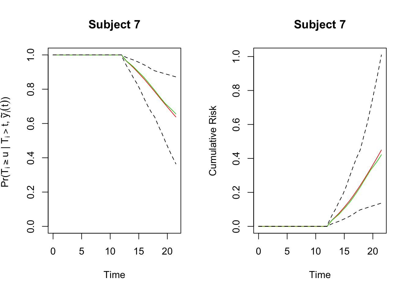
The CD4 cell counts are known to exhibit right skewed shapes of distribution, and therefore, for the remainder of this analysis we will work with the square root of the CD4 cell values.↩