3.5 Adjusting Survival Curves

From a survival analysis point of view, we want to obtain also estimates for the survival curve. Remember that if we do not use a model, we can apply the Kaplan-Meier estimator. However, when a Cox model is used to fit survival data, survival curves can be obtained adjusted for the explanatory variables used as predictors. These are called adjusted survival curves and, like Kaplan-Meier curves, these are also plotted as step functions.

The hazard formula seen before can be converted to a survival function as

\[ S(t|\textbf X) = \bigg[ S_0(t) \bigg]^{e^{\sum_{j=1}^p \beta_j X_j}}. \]

This survival function formula is the basis for determining adjusted survival curves. The estimates of \(\hat S_0(t)\) and \(\hat b_j\) are provided by the computer program that fits the Cox model. The \(X\)’s, however, must first be specified by the investigator before the computer program can compute the estimated survival curve.

Typically, when computing adjusted survival curves, the value chosen for a covariate being adjusted is an average value like an arithmetic mean or a median.

The survfit function estimates \(S(t)\), by default at the mean values of the covariates:

m2 <- m_red
newdf <- data.frame(IsBorrowerHomeowner = levels(loan_filtered$IsBorrowerHomeowner), 
                    LoanOriginalAmount2 = rep(mean(loan_filtered$LoanOriginalAmount2), 2))
fit <- survfit(m2, newdata = newdf)
#summary(fit) # to see the estimated values
plot(fit, conf.int = TRUE, col = c(1,2))
legend("bottomleft", levels(newdf[,1]), col = c(1, 2), lty = c(1,1))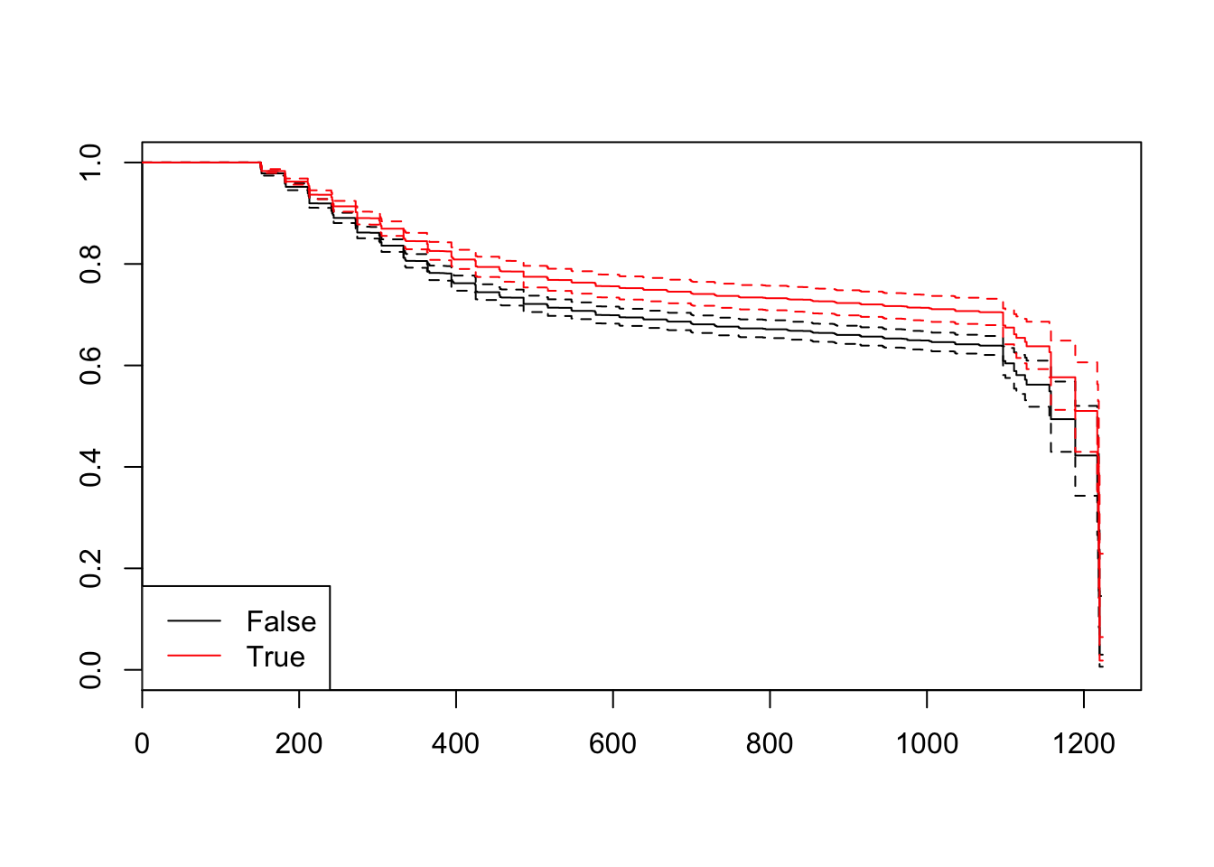

# another option using the survminer package
survminer::ggsurvplot(fit, data = newdf)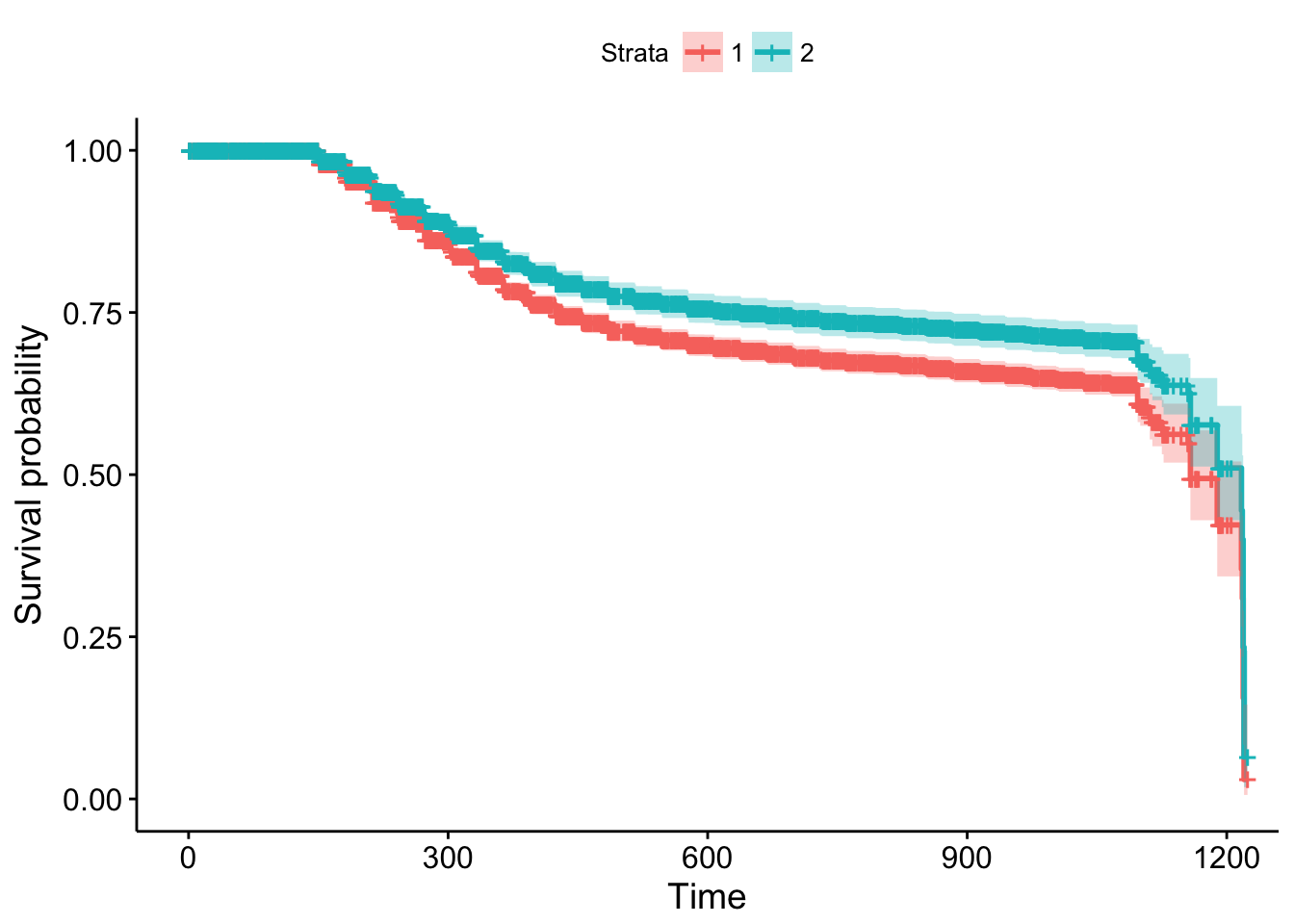

# easier... without refitting
#survminer::ggadjustedcurves(m2, data = loan_filtered, 
#                    variable = loan_filtered$IsBorrowerHomeowner)

For some help with the survminer package… Download the cheatsheet here.

Try to estimate a Cox PH model using your dataset.