4.1 Linear Mixed Models
As we mentioned, Joint Models take two outcomes into account, the longitudinal response and the survival time. In order to estimate these type of models, we need first to fit a model for the longitudinal response (usually a linear mixed model) and then for the survival time.
I am assuming here that you have understood entirely the Chapter 3 and you do not have any problem with the estimation of the Cox model by means of the coxph function. Regarding the linear mixed model you can see an brief introduction with examples below using the nlme package. For a good overview you can consult the Chapter 2 of Rizopoulos (2012).
So, our focus in this part is on longitudinal data. This data can be defined as the data resulting from the observations of subjects (e.g., human beings, animals, etc.) that are measured repeatedly over time. From this descriptions, it is evident that in a longitudinal setting we expect repeated measurements taken on the same subject to exhibit positive correlation. This feature implies that standard statistical tools, such as the t-test and simple linear regression that assume independent observations, are not appropriate for longitudinal data analysis (they may produce invalid standard errors). In order to solve this situation and obtain valid inference, one possible approach is to use a mixed model, a regression method for continuous outcomes that models longitudinal data by assuming, for example, random errors within a subject and random variation in the trajectory among subjects.
We are going to explain briefly this approach. Figure 4.1 shows an example with hypothetical longitudinal data for two subjects. In this figure, monthly observations are recorded for up to one year. Note that each subject appears to have their own linear trajectory but with small fluctuations about the line. This fluctuations are referred to as the within-subject variation in the outcomes. Note that if we only have data from one person these will be the typical error term in regression. The dashed line in the center of the figure shows the average of individual linear-time trajectories. This line characterizes the average for the population as a function of time. For example, the value of the dashed line at month 2 is the mean response if the observation (at two months) for all subjects was averaged. Thus, this line represents both the typical trajectory and the population average as a function of time.
The main idea of Linear Mixed Model is that they make specific assumptions about the variation in observations attributable to variation within a subject and to variation among subjects. To formally introduce this representation of longitudinal data, we let \(Y_{ij}\) denote the response of subject \(i, i = 1, \ldots, n\) at time \(X_{ij}, j = 1,...,n_i\) and \(\beta_{i0} + \beta_{i1} X_{ij}\) denote the line that characterizes the observation path for \(i\). Note that each subject has an individual-specific intercept and slope. Note that
The within-subject variation is seen as the deviation between individual observations, \(Y_{ij}\), and the individual linear trajectory, that is \(Y_{ij} - (\beta_{i0} + \beta_{i1} X_{ij})\).
The between-subject variation is represented by the variation among the intercepts, \(var(\beta_{i0})\) and the variation among subject in the slopes \(var(\beta_{i1})\).
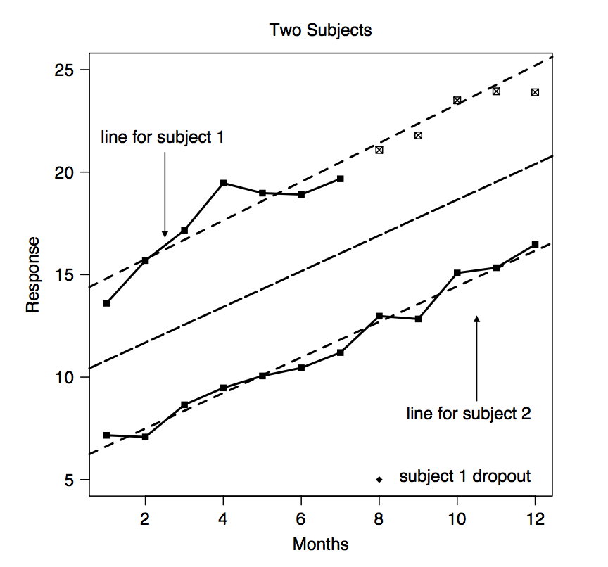
Figure 4.1: Hypothetical longitudinal data for two subjects.
Figure 4.1 taken from Belle et al. (2004).
If parametric assumptions are made regarding the within- and between-subject components of variation, it is possibel to use maximum likelihood methods for estimating the regression parameters (which characterize the population average), and the variance components (which characterize the magnitude of within- and between-subject heterogeneity). For continuous outcomes it is a good idea to assume that within-subject errors are normally distributed and to assume that intercepts and slopes are normally distributed among subjects. This will be
- within-subjects: \[ E(Y_{ij}|\beta_i) = \beta_{i,0} + \beta_{i, 1} X_{ij} \]
\[ Y_{ij} = \beta_{i,0} + \beta_{i, 1} X_{ij} + \varepsilon_{ij} \]
\[ \varepsilon_{ij} \sim N(0, \sigma^2) \]
- between-subjects:
\[ \bigg(\begin{array}{c} \beta_{i,0}\\ \beta_{i,1}\\ \end{array} \bigg) \sim N \bigg[ \bigg(\begin{array}{c} \beta_{0}\\ \beta_{1}\\ \end{array} \bigg), \bigg(\begin{array}{c} D_{00} & D_{01}\\ D_{10} & D_{11}\\ \end{array} \bigg) \bigg] \] where \(D\) is the variance-covariance matrix of the random effects, with \(D_{00}= var(b_{i,0})\) and \(D_{11}= var(b_{i,1})\).
If we think in \(b_{i,0}= (\beta_{i,0} - \beta_0)\) and \(b_{i,1}= (\beta_{i,1} - \beta_1)\), the model can be written as
\[ Y_{ij} = \beta_0 + \beta_1 X_{ij} + b_{i,0} + b_{i,1} X_{ij} + \varepsilon_{ij} \] where \(b_{i,0}\) and \(b_{i,1}\) represent deviations from the population average intercept and slope respectively.
Note taht in this equation there is a systematic variation (given by the two first betas) and a random variation (the rest). Additionally, the random component is partitioned into the observation level and subject level fluctuations: that is, the between-subject (\(b_{i,0} + b_{i,1} X_{ij}\)) and within-subject (\(\varepsilon_{ij}\)) variations.
A more general form including \(p\) predictors is
\[ Y_{ij} = \beta_0 + \beta_1 X_{ij,1} +\ldots + + \beta_p X_{ij,p} + b_{i,0} + b_{i,1} X_{ij,1} + \ldots + b_{i,p} X_{ij,p}+ \varepsilon_{ij} \]
\[ Y_{ij} = X_{ij}'\beta + Z_{ij}' b_i + \varepsilon_{ij} \] where \(X_{ij}'=[X_{ij,1}, X_{ij,2}, \ldots, X_{ij,p}]\) and \(Z_{ij}'=[X_{ij,1}, X_{ij,2}, \ldots, X_{ij,q}]\). In general way, we assume that the covariates in \(Z_{ij}\) are a subset of the variables in \(X_{ij}\) and thus \(q < p\).
Moving again onto the example, it seems that each subject has their own intercept, but the subjects may have a common slope. So, a random intercept model assumes parallel trajectories for any two subjects and is given as a special case of the general mixed model:
\[ Y_{ij} = \beta_0 + \beta_1 X_{ij,1} + b_{i,0} + \varepsilon_{ij}. \]
Using the above model, the intercept for subject \(i\) is given by \(\beta_0 + b_{i,0}\) while the slope for subject \(i\) is simply \(\beta_1\) since there is no additional random slope, \(b_{i,1}\) in the random intercept model.
If we assume that the slope for each individual \(i\) can also be different, we have to use a random intercept and slope model of the type
\[ Y_{ij} = \beta_0 + \beta_1 X_{ij,1} + b_{i,0} + b_{i,1} X_{ij,1}+ \varepsilon_{ij}. \] and now the intercept for subject \(i\) is given by \(\beta_0 + b_{i,0}\) while the slope for subject \(i\) is \(\beta_1 + b_{i, 1}\).
In order to fit these models, we can use the lme function of the nlme package.
head(aids)
##   patient  Time death       CD4 obstime drug gender prevOI         AZT
## 1       1 16.97     0 10.677078       0  ddC   male   AIDS intolerance
## 2       1 16.97     0  8.426150       6  ddC   male   AIDS intolerance
## 3       1 16.97     0  9.433981      12  ddC   male   AIDS intolerance
## 4       2 19.00     0  6.324555       0  ddI   male noAIDS intolerance
## 5       2 19.00     0  8.124038       6  ddI   male noAIDS intolerance
## 6       2 19.00     0  4.582576      12  ddI   male noAIDS intolerance
##   start  stop event
## 1     0  6.00     0
## 2     6 12.00     0
## 3    12 16.97     0
## 4     0  6.00     0
## 5     6 12.00     0
## 6    12 18.00     0
# CD4: square root CD4 cell count measurements
# obstime: time points at which the corresponding longitudinal response was recorded
# random-intercepts model (single random effect term for each patient)
fit1 <- lme(fixed = CD4 ~ obstime, random = ~ 1 | patient, data = aids)
summary(fit1)
## Linear mixed-effects model fit by REML
## Data: aids
## AIC BIC logLik
## 7176.633 7197.618 -3584.316
##
## Random effects:
## Formula: ~1 | patient
## (Intercept) Residual
## StdDev: 4.506494 1.961662
##
## Fixed effects: CD4 ~ obstime
## Value Std.Error DF t-value p-value
## (Intercept) 7.188663 0.22061320 937 32.58492 0
## obstime -0.148500 0.01218699 937 -12.18513 0
## Correlation:
## (Intr)
## obstime -0.194
##
## Standardized Within-Group Residuals:
## Min Q1 Med Q3 Max
## -3.84004681 -0.44310988 -0.05388055 0.43593364 6.09265321
##
## Number of Observations: 1405
## Number of Groups: 467Note that the estimation for the variability or the variance components, that is, the variance of the errors (\(\varepsilon_{ij}\), within personal errors) and the variance between subject (the variance of the \(b_{i, 0}\)) are given under Random effects heading. Under (Intercept) we can see the estimated standard desviation for the \(b_{i,0}\) coefficients and under Residual, the estimated desviation for \(\varepsilon_{ij}\).
# variance of the beta_i0
getVarCov(fit1)
## Random effects variance covariance matrix
##             (Intercept)
## (Intercept)      20.308
##   Standard Deviations: 4.5065

# standard desviation of e_ij
fit1$sigma
## [1] 1.961662

# total variance of the model
getVarCov(fit1)[1] + fit1$sigma**2
## [1] 24.15661

# % variance within person
(fit1$sigma**2/(getVarCov(fit1)[1] + fit1$sigma**2)) * 100
## [1] 15.92988

# % variance between person
(getVarCov(fit1)[1]/(getVarCov(fit1)[1] + fit1$sigma**2)) * 100
## [1] 84.07012
The total variation in CD4 is estimated as 24.16. So, the proportion of total variation that is attributed to within-person variability is 15.93% with 84.07% of total variation attributable to individual variation in their general level of CD4 (attributable to random intercepts).
The estimated regression coefficients \(\beta\) are provided under the Fixed effects heading. As expected, the coefficient for the time effect has a negative sign indicating that on average the square root CD4 cell counts declines in time.
Well, this random-intercepts model poses the unrealistic restriction that the correlation between the repeated measurements remains constant over time (we are not includiying the random slope yet). So, a natural extension is a more flexible specification of the covariance structure with the random-intercepts and random-slopes model. This model introduces an additional random effects term, and assumes that the rate of change in the CD4 cell count is different from patient to patient.
# random-intercepts and random-slopes model
fit2 <- lme(CD4 ~ obstime, random = ~ obstime | patient, data = aids) # the intercept is  included by default
summary(fit2)
## Linear mixed-effects model fit by REML
##  Data: aids
##        AIC     BIC    logLik
##   7141.282 7172.76 -3564.641
##
## Random effects:
##  Formula: ~obstime | patient
##  Structure: General positive-definite, Log-Cholesky parametrization
##             StdDev    Corr
## (Intercept) 4.5898645 (Intr)
## obstime     0.1728724 -0.152
## Residual    1.7507904
##
## Fixed effects: CD4 ~ obstime
##                 Value  Std.Error  DF  t-value p-value
## (Intercept)  7.189048 0.22215494 937 32.36051       0
## obstime     -0.150059 0.01518146 937 -9.88435       0
##  Correlation:
##         (Intr)
## obstime -0.218
##
## Standardized Within-Group Residuals:
##         Min          Q1         Med          Q3         Max
## -4.31679141 -0.41425035 -0.05227632  0.41094183  4.37413201
##
## Number of Observations: 1405
## Number of Groups: 467
We observe very minor differences in the estimated fixed-effect parameters compared with the previous model. Maybe the AIC For example, for the random effects, we can observe that there is greater variability between patients in the baseline levels of CD4 (given by (Intercept) variance) than in the evolutions of the marker in time (obstime variance).
anova(fit1, fit2) # reduced vs full
##      Model df      AIC      BIC    logLik   Test  L.Ratio p-value
## fit1     1  4 7176.633 7197.618 -3584.316
## fit2     2  6 7141.282 7172.760 -3564.641 1 vs 2 39.35067  <.0001

# it is better to use the random-intercepts and random-slopes model
muhat <- predict(fit2)
aids2 <- aids
aids2$muhat <- muhat
lattice::xyplot(muhat ~ obstime, group = patient,
data = aids2[aids2$patient %in% c(1:10), ],type = "l")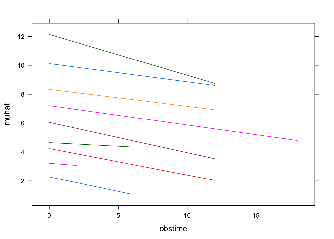
References
Rizopoulos, Dimitris. 2012. Joint Models for Longitudinal and Time-to-Event Data: With Applications in R. 1st ed. Chapman & Hall/Crc Biostatistics Series. Chapman; Hall/CRC. http://gen.lib.rus.ec/book/index.php?md5=99C084286F029FD36E10FE18AA587A7C.
Belle, Gerald van, Lloyd D. Fisher, Patrick J. Heagerty, and Thomas Lumley. 2004. Biostatistics: A Methodology for the Health Sciences. Wiley Online Library.