1.4 Survival/hazard functions
Assuming that \(T\) is a continuous non-negative random variable which denote the time-to-event. There is a certain probability that an individual will have an event at exactly time \(t\). For example, about human longevity, human beings have a certain probability of dying at ages \(2\), \(20\), \(80\), and \(140\), that could be: \(P(T=2)\), \(P(T=20)\), \(P(T=80)\) and \(P(T=140)\).
Similarly, human beings have a certain probability of being alive at those same ages: \(P(T>2)\), \(P(T>20)\), \(P(T>80)\), and \(P(T>140)\).
Here an example with same real data:1
data <- read.table("data/deaths_esp.txt", header = TRUE, sep = "")
data <- data[!data$Age == "110+", ] # to avoid errors
data$Age_cut <- cut(as.numeric(as.character(data$Age)),
                 breaks =  seq(0,110, 10), right = FALSE)

by_age <- data %>%
  group_by(Age_cut)  %>%
  summarise (sum_deaths = sum(Total, na.rm = TRUE))

barplot(by_age$sum_deaths/sum(data$Total), names.arg = by_age$Age_cut, ylab= "Relative frequency") 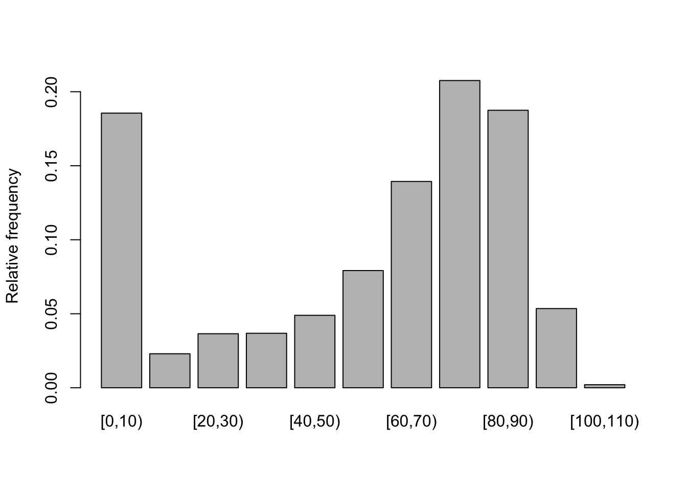
Figure 1.2: Relative frequiencies for grouped ages.
In the case of human longevity, the probability of death is higher at the beginning and end of life (in Spain). Therefore, \(T\) is unlikely to follow a normal distribution. We can see a higher chance of dying (the event of interest) in their 70’s and 80’s and smaller chance of dying in their 100’s and 110’s, because few people make it long enough to die at these age.
The function that gives the probability of the failure time occurring at exactly time \(t\) is the density function \(f(t)\)2
\[ f(t) = \displaystyle{lim_{\Delta_t \to 0}} \frac{P(t \le T < t + \Delta t)}{\Delta t} \] and the function that gives the probability of the failure time occur before or exactly at time \(t\) is the cumulative distribution function \(F(t)\)
\[ F(t) = P(T \le t) = \int_{0}^{t} f(u) du. \]
Note that \(F(t)\) is more interesting than \(f(t)\)… And why? Well, as we said, the main goal of survival analysis is to estimate and compare survival experiences of different groups and the survival experience is described by the survival function \(S(t)\)
\[ S(t) = P(T > t) = 1 - F(t) \]
The survival function gives the probability that a person survives longer than some specified time \(t\): that is, \(S(t)\) gives the probability that the random variable \(T\) exceeds the specified time \(t\). And here, some important characteristics:
It is nonincreasing; that is, it heads downward as \(t\) increases.
At time \(t = 0\), \(S(t) = S(0)= 1\); that is, at the start of the study, since no one has gotten the event yet, the probability of surviving past time zero is one.
At time \(t = \inf\), \(S(t) = S(\inf) = 0\); that is, theoretically, if the study period increased without limit, eventually nobody would survive, so the survival curve must eventually fall to zero.
t <- seq(0, 110, 1)
tdf <- pweibull(t, scale = 80, shape = 5) # weibull dist

d <- reshape2::melt(data.frame(x = t, dist = tdf, surv = 1 - tdf), id = "x")
qplot(x = x, y = value, col = variable, data = d, geom = "line",
      ylab = "probability", xlab = "t") +
scale_colour_discrete(labels= c("F(t)", "S(t)"), name = "") 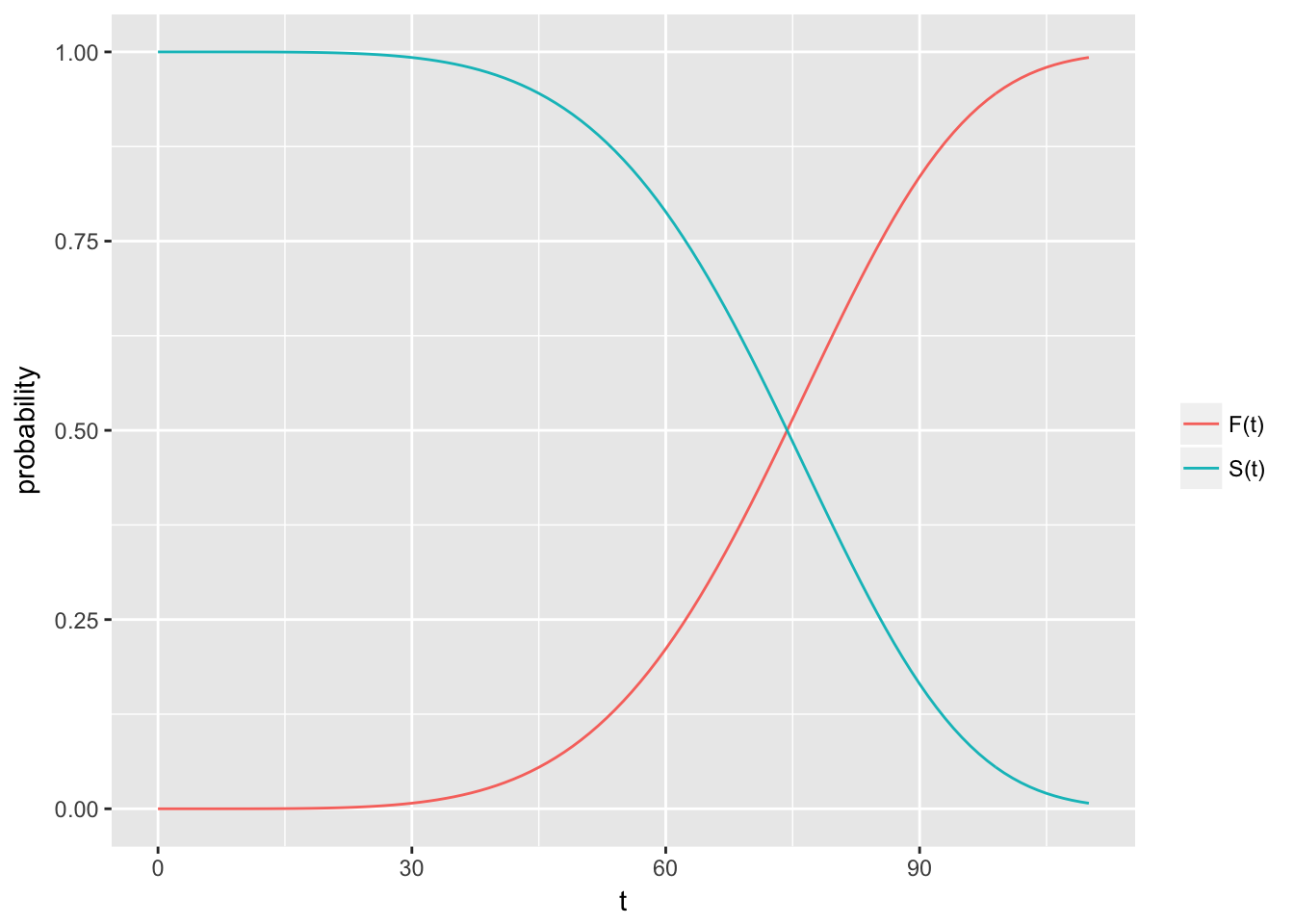
Note that these are theoretical properties of survival curves. In practice, when using actual data, we usually obtain graphs that are step functions, rather than smooth curves. Moreover, because the study period is never infinite in length and there may be competing risks for failure, it is possible that not everyone studied gets the event. The estimated survival function, \(\hat{S}(t)\) thus may not go all the way down to zero at the end of the study.
by_age <- data %>%
  group_by(Age)  %>%
  summarise (sum_deaths = sum(Total, na.rm = T))
t <- rep(as.numeric(as.character(by_age$Age)), by_age$sum_deaths) # real times

aux <- ecdf(t)
x <- seq(0, 110, 1)
edf <- aux(x) # evaluating the ecdf in some points
esf <- 1- edf

d <- reshape2::melt(data.frame(x = x, dist = edf, surv = esf), id = "x")
qplot(x = x, y = value, col = variable, data = d, geom = "step",
      ylab = "Probability", xlab = "t") + scale_colour_discrete(labels = c("F(t)", "S(t)"), name = "")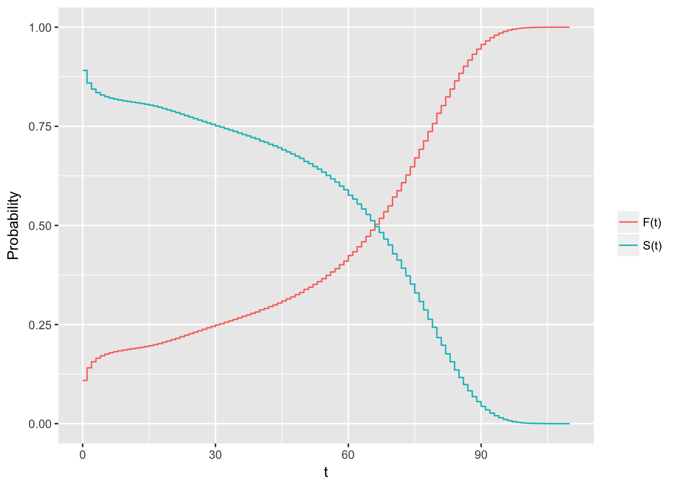
The hazard function \(h(t)\), is given by the formula:
\[ h(t) = \displaystyle{lim_{\Delta_t \to 0}} \frac{P(t \le T < t + \Delta t | T \ge t)}{\Delta t} \] This mathematical formula is difficult to explain in practical terms. We could say that the hazard function is the probability that if you survive to time \(t\), you will experience the event in the next instant, or in other words, the hazard function gives the instantaneous potential per unit time for the event to occur, given that the individual has survived up to time \(t\). Because of the given sign here, the hazard function is sometimes called a conditional failure rate.
Note that, in contrast to the survival function, which focuses on not failing, the hazard function focuses on failing, that is, on the event occurring. Thus, in some sense, the hazard function can be considered as giving the opposite side of the information given by the survivor function.
Additionally, in contrast to a survival function, the graph of \(h(t)\) does not have to start at one and go down to zero, but rather can start anywhere and go up and down in any direction over time. In particular, for a specified value of \(t\), the hazard function \(h(t)\) has the following characteristics:
It is always nonnegative, that is, equal to or greater than zero.
It has no upper bound.
Finally note that the hazard function can be expressed as the probability density function divided by the survival function, \(h(t) = \frac{f(t)}{S(t)}\):
\[ P(t \le T \lt t + dt | T \ge t) = \frac{P(t \le T \lt t + dt, T \ge t)}{P(T \ge t)} = \frac{P(t \le T \lt t + dt)}{P(T \ge t)} \]
h <- hist(t, plot = FALSE)
x <- h$mids
dens <- h$density
surv <- 1 - aux(x)
hazard <- dens/surv
qplot(x = x, y = hazard, geom = "line", ylab = "Conditional probability of death",
      xlab = "Age")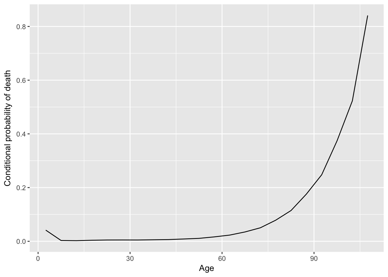
In some cases it can be more interesting to present the cumulative hazard. It will be \(H(t) = \int_{0}^{t} h(u) du\).
Hazard vs. density function
According to the human longevity study, note that when you are born, you have a certain probability of dying at any age, that will be \(P(T = t)\), i.e. the density function. A woman born today has, say, a 1% chance of dying at 80 years. However, as you survive for a while, your probabilities keep changing, and these new conditional probabilities are given by the hazard function. In such case, we have a woman who is 79 today and has, say, a 7% chance of dying at 80 years.Data from The Human Mortality Database at http://www.mortality.org.↩
The probability mass function is a function that gives the probability that a discrete random variable is exactly equal to some value.↩