3.9 Bonus track 1: Additive Cox model

The Cox PH model assumes a linear effect of the predictors. If the true effect is highly nonlinear this can lead to a nonproportinal hazards or misleading statistical conclusions.

One alternative approach is to use an Additive Cox model (Hastie and Tibshirani 1990) of the form

\[ h(t, \textbf X) = h_0(t) e^{\sum_{j=1}^p f_j(\textbf X_j)} \] with \(f_j\) being an unknown and smooth function.

In order to estimate this model one could use the mgcv package as follows

m4 <- mgcv::gam(time ~ s(LoanOriginalAmount2) + IsBorrowerHomeowner, 
                data = loan_filtered, family = "cox.ph", weights = status)
summary(m4)
## 
## Family: Cox PH 
## Link function: identity 
## 
## Formula:
## time ~ s(LoanOriginalAmount2) + IsBorrowerHomeowner
## 
## Parametric coefficients:
##                         Estimate Std. Error z value Pr(>|z|)    
## IsBorrowerHomeownerTrue -0.23344    0.06248  -3.736 0.000187 ***
## ---
## Signif. codes:  0 '***' 0.001 '**' 0.01 '*' 0.05 '.' 0.1 ' ' 1
## 
## Approximate significance of smooth terms:
##                          edf Ref.df Chi.sq  p-value    
## s(LoanOriginalAmount2) 4.853  5.857  26.91 0.000206 ***
## ---
## Signif. codes:  0 '***' 0.001 '**' 0.01 '*' 0.05 '.' 0.1 ' ' 1
## 
## Deviance explained = 0.818%
## -REML =  10848  Scale est. = 1         n = 4923
plot(m4, pages = 1, all.terms = TRUE)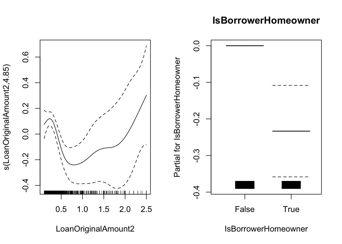

Note the change in the sintaxis compared with the previous examples. The status indicator in used in the weights argument.

References

Hastie, T., and R. Tibshirani. 1990. Generalized Additive Models. London: Chapman; Hall.