6.3 Aplication to real data
head(veteran)
##   trt celltype time status karno diagtime age prior
## 1   1 squamous   72      1    60        7  69     0
## 2   1 squamous  411      1    70        5  64    10
## 3   1 squamous  228      1    60        3  38     0
## 4   1 squamous  126      1    60        9  63    10
## 5   1 squamous  118      1    70       11  65    10
## 6   1 squamous   10      1    20        5  49     0

fit <- survfit(Surv(time, status) ~ factor(celltype), data = veteran)
autoplot(fit)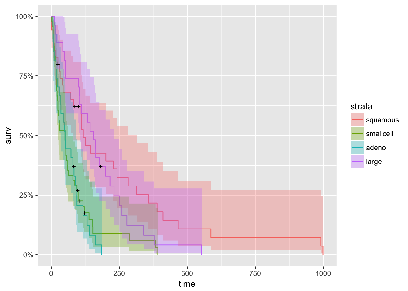
survdiff(Surv(time,status)~factor(celltype), data=veteran)
## Call:
## survdiff(formula = Surv(time, status) ~ factor(celltype), data = veteran)
##
##                             N Observed Expected (O-E)^2/E (O-E)^2/V
## factor(celltype)=squamous  35       31     47.7      5.82     10.53
## factor(celltype)=smallcell 48       45     30.1      7.37     10.20
## factor(celltype)=adeno     27       26     15.7      6.77      8.19
## factor(celltype)=large     27       26     34.5      2.12      3.02
##
##  Chisq= 25.4  on 3 degrees of freedom, p= 1.27e-05
survminer::pairwise_survdiff(Surv(time, status) ~ celltype,
                                    data = veteran, p.adjust.method = "BH")
##
##  Pairwise comparisons using Log-Rank test
##
## data:  veteran and celltype
##
##           squamous smallcell adeno
## smallcell 0.00134  -         -
## adeno     0.00134  0.75565   -
## large     0.43731  0.00331   0.00016
##
## P value adjustment method: BH

?clustcurv_surv
res <- clustcurv_surv(time = veteran$time, status = veteran$status,
                      fac = veteran$celltype, algorithm = "kmeans",
                      nboot = 100,
                      cluster = TRUE, seed = 29072016)
## Checking 1 cluster...
## Checking 2 clusters...
##
## Finally, there are 2 clusters.
res
## $table
##   H0    Tvalue pvalue
## 1  1 3.2108812   0.00
## 2  2 0.3799373   0.43
##
## $levels
## [1] "squamous"  "smallcell" "adeno"     "large"
##
## $cluster
## [1] 2 1 1 2
##
## $centers
## Call: survfit(formula = Surv(time, status) ~ aux$cluster[fac])
##
##                     n events median 0.95LCL 0.95UCL
## aux$cluster[fac]=1 75     71     51      30      73
## aux$cluster[fac]=2 62     57    143     110     216
##
## $curves
## Call: survfit(formula = Surv(time, status) ~ fac)
##
##                n events median 0.95LCL 0.95UCL
## fac=squamous  35     31    118      82     314
## fac=smallcell 48     45     51      25      63
## fac=adeno     27     26     51      35      92
## fac=large     27     26    156     105     231
##
## attr(,"class")
## [1] "clustcurv_surv"

autoplot(res, groups_by_colour = TRUE, xlab = "Time (in days)")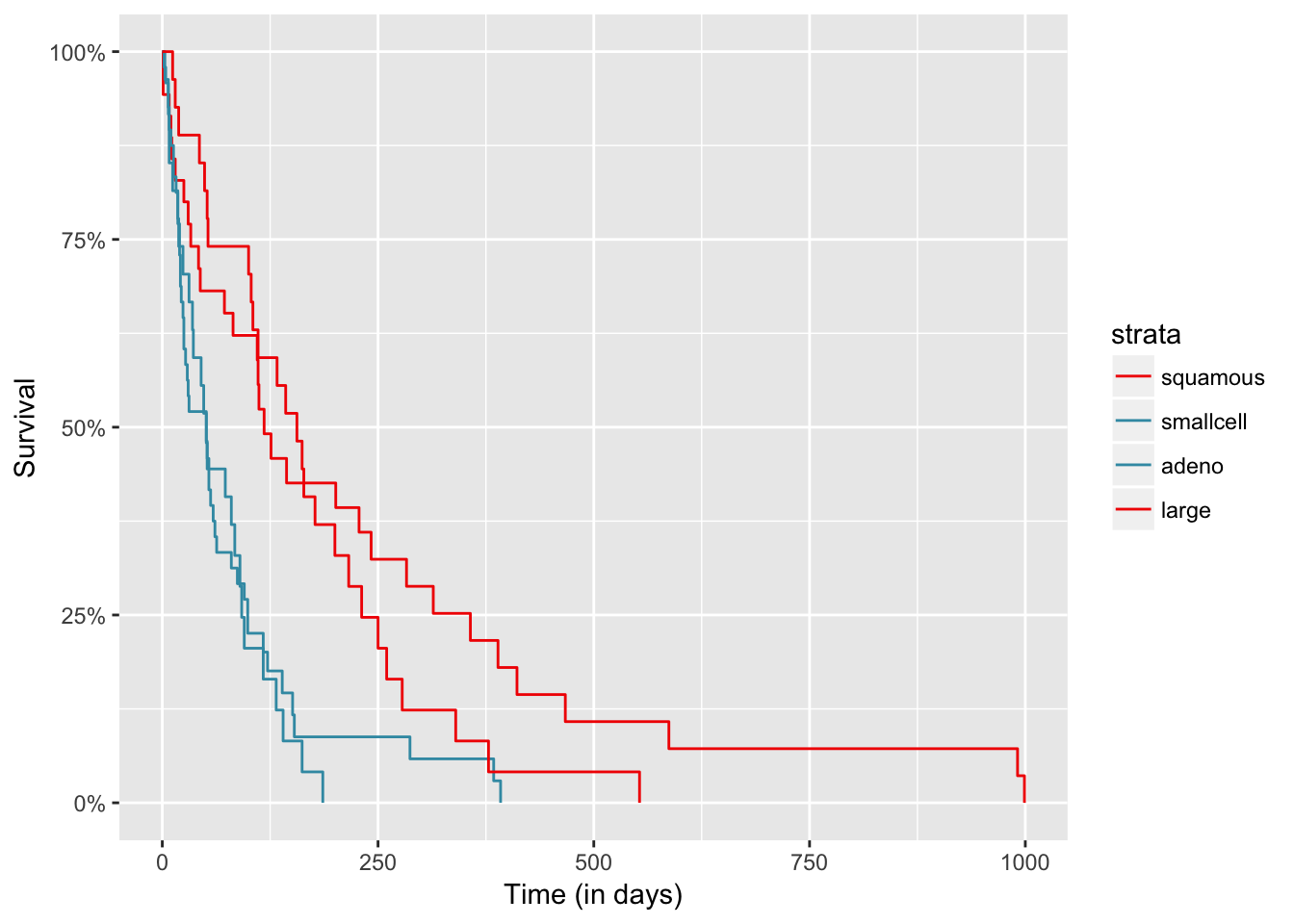
Now we are going to see anoyher example with a catgorical variable with more levels.
colonCSm <- na.omit(data.frame(time = colonCS$Stime, status = colonCS$event,
                       nodes = colonCS$nodes))
table(colonCSm$nodes)
##
##   0   1   2   3   4   5   6   7   8   9  10  11  12  13  14  15  16  17
##   2 274 194 125  84  46  43  38  23  20  13  10  11   7   4   6   1   2
##  19  20  22  24  27  33
##   2   2   1   1   1   1
# deleting people with zero nodes
colonCSm <- colonCSm[-c(which(colonCSm$nodes == 0)), ]
table(colonCSm$nodes)
##
##   1   2   3   4   5   6   7   8   9  10  11  12  13  14  15  16  17  19
## 274 194 125  84  46  43  38  23  20  13  10  11   7   4   6   1   2   2
##  20  22  24  27  33
##   2   1   1   1   1

# grouping people with more than 10 nodes
colonCSm$nodes[colonCSm$nodes >= 10] <- 10
table(colonCSm$nodes)  # 10 levels
##
##   1   2   3   4   5   6   7   8   9  10
## 274 194 125  84  46  43  38  23  20  62


model <- survfit(Surv(time, status) ~ factor(nodes), data = colonCSm)
survdiff(Surv(time,status)~factor(nodes), data = colonCSm)
## Call:
## survdiff(formula = Surv(time, status) ~ factor(nodes), data = colonCSm)
##
##                    N Observed Expected (O-E)^2/E (O-E)^2/V
## factor(nodes)=1  274       94   151.93   22.0901   33.9249
## factor(nodes)=2  194       74   102.87    8.1022   10.5979
## factor(nodes)=3  125       61    62.56    0.0387    0.0453
## factor(nodes)=4   84       43    38.26    0.5868    0.6434
## factor(nodes)=5   46       34    17.06   16.8249   17.5428
## factor(nodes)=6   43       27    16.43    6.8027    7.0736
## factor(nodes)=7   38       25    15.41    5.9636    6.1880
## factor(nodes)=8   23       18     7.22   16.0875   16.3765
## factor(nodes)=9   20       14     8.05    4.3931    4.4795
## factor(nodes)=10  62       49    19.21   46.2239   48.6066
##
##  Chisq= 129  on 9 degrees of freedom, p= 0


survminer::pairwise_survdiff(Surv(time, status) ~ nodes,
                                    data = colonCSm, p.adjust.method = "BH")
##
##  Pairwise comparisons using Log-Rank test
##
## data:  colonCSm and nodes
##
##    1       2       3       4       5       6       7       8       9
## 2  0.41644 -       -       -       -       -       -       -       -
## 3  0.00853 0.10482 -       -       -       -       -       -       -
## 4  0.00221 0.04032 0.51450 -       -       -       -       -       -
## 5  3.9e-09 1.8e-06 0.00072 0.03427 -       -       -       -       -
## 6  1.7e-05 0.00072 0.03750 0.22540 0.60307 -       -       -       -
## 7  2.1e-05 0.00072 0.04219 0.25752 0.49274 0.95088 -       -       -
## 8  3.0e-08 4.1e-06 0.00047 0.01407 0.51450 0.30796 0.25752 -       -
## 9  0.00043 0.00493 0.08152 0.23872 0.76034 0.90717 0.79064 0.51450 -
## 10 < 2e-16 1.2e-11 9.1e-07 0.00047 0.37154 0.16671 0.10386 0.95088 0.37007
##
## P value adjustment method: BH


res <- clustcurv_surv(time = colonCSm$time, status = colonCSm$status,
                      fac = colonCSm$nodes, algorithm = "kmeans",
                      nboot = 100, cluster = TRUE, seed = 300716)
## Checking 1 cluster...
## Checking 2 clusters...
##
## Finally, there are 2 clusters.

autoplot(res, groups_by_colour = FALSE, xlab = "Time (in days)")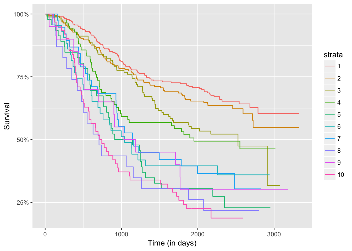
autoplot(res, groups_by_colour = TRUE, xlab = "Time (in days)")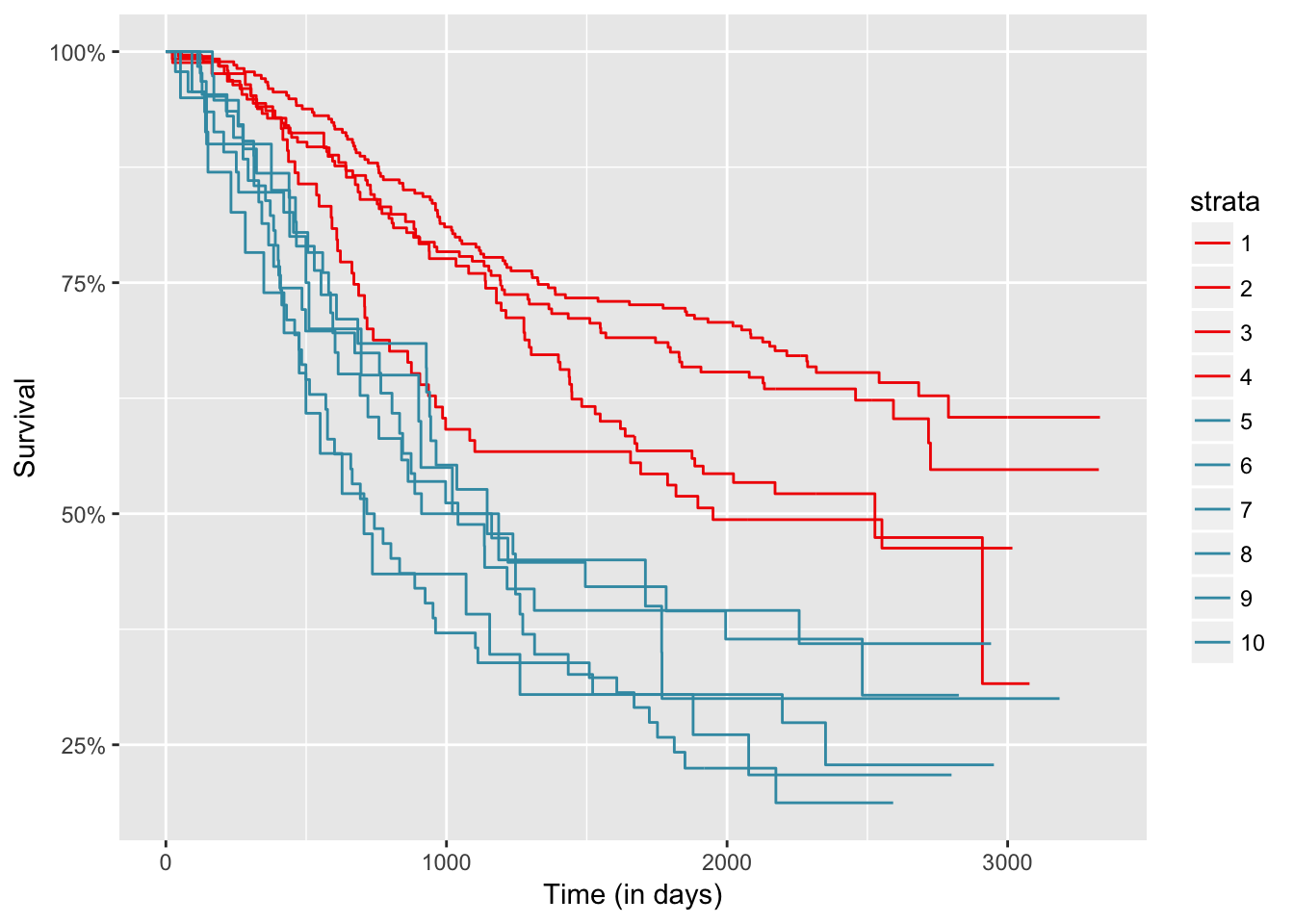
res$table
## H0 Tvalue pvalue
## 1 1 15.425589 0.00
## 2 2 2.364531 0.18
data.frame(res$levels, res$cluster)
## res.levels res.cluster
## 1 1 2
## 2 2 2
## 3 3 2
## 4 4 2
## 5 5 1
## 6 6 1
## 7 7 1
## 8 8 1
## 9 9 1
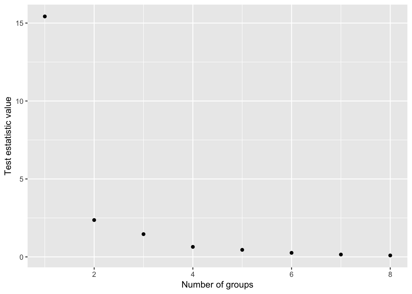
## 10 10 1One faster option than applying directly the `clustcurv_surv` function, that is based on boostrap techniques for detecting the number of groups, is to use the `kgroups_surv` for $k = 1, \ldots, J-1$. Then you can plot the resulted measures for each $k$ and choose the one that with the "less" measure.fun <- function(x){
kgroups_surv(time = colonCSm$time, status = colonCSm$status,
fac = colonCSm$nodes, algorithm = "kmeans", k = x)$measure
}
ts <- sapply(1:8, fun)
qplot(1:8, ts, xlab = "Number of groups", ylab = "Test estatistic value")