2.3 Comparing survival curves
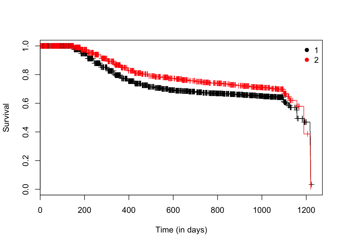
As we have seen before, we can use the survfit function to estimate the survival using the Kaplan-Meier estimator taking into account the censored data. Additionally, it is possible to include a factor in the model and to obtain the estimated survival for each of the levels of the factor.
model <- survfit(Surv(time, status) ~ IsBorrowerHomeowner, data = loan_filtered)
plot(model, ylab = "Survival", xlab = "Time (in days)", col = 1:2, mark.time = TRUE)
legend("topright", col = 1:2, legend =
         levels(factor(lung$sex)),
       bty = "n", pch = 19)
Now, the questions that arises is if these two curves are statistivally equivalent. For answering it, we can use the log-rank test (Mantel 1966; Peto and Peto 1972). This is the most well-known and widely used method to test the null hypothesis of no difference in survival between two or more independent groups. It is a large-sample chi-square test that is obtained by constructing a two by two contingency table at each distinct event time, and comparing the failure rates between the two groups, conditional on the number at risk in each group. The test compares the entire survival experience between groups and can be thought of as a test of whether the survival curves are identical or not.
The null hypothesis (\(H_0\)) of the testing procedure is that there is no overall difference between the two (or \(k\)) survival curves. Under this \(H_0\), the log–rank statistic is approximately a chi-square with \(k-1\) degree of freedom. Thus, tables of the chi-square distribution are used to determine the pvalue.
This test is the one with most power to test differences that fit the proportional hazards model - so works well as a set-up for subsequent Cox regression. It gives equal weight to early and late failures.
An alternative test that is often used is the Peto & Peto (Peto and Peto 1972) modification of the Gehan-Wilcoxon test (Gehan 1965). This last one is a variation of the log-rank test statistic and is derived by applying different weights at the \(f-\)th failure time. This approach is most sensitive to early differences (or earlier time points) between survival.
This type of weighting may be used to assess whether the effect of a treatment/marketing campaing on survival is strongest in the earlier phases of administration/contacto and tends to be less effective over time.
In the absence of censoring, these methods reduce to the Wilcoxon-Mann-Whitney rank-sum test (Mann and Whitney 1947) for two samples and to the Kruskal-Wallis test (Kruskal and Wallis 1952) for more than two groups of survival times.
Of course, several other variations of the log-rank test statistic using weights on each event time have been proposed in the literature [Tarone and Ware (1977); doi:10.1093/biomet/69.3.553; 10.2307/2289169].
The log-rank test and the Peto & Peto modification of the log-rank test are both implemented in the survdiff function in library survival.
survdiff(Surv(time, status) ~ IsBorrowerHomeowner, data = loan_filtered, rho = 0) # log-rank
## Call:
## survdiff(formula = Surv(time, status) ~ IsBorrowerHomeowner,
##     data = loan_filtered, rho = 0)
##
##                              N Observed Expected (O-E)^2/E (O-E)^2/V
## IsBorrowerHomeowner=False 3342     1001      926      6.13      19.4
## IsBorrowerHomeowner=True  1581      362      437     12.98      19.4
##
##  Chisq= 19.4  on 1 degrees of freedom, p= 1.04e-05

survdiff(Surv(time, status) ~ IsBorrowerHomeowner, data = loan_filtered, rho = 1)# peto & peto
## Call:
## survdiff(formula = Surv(time, status) ~ IsBorrowerHomeowner,
##     data = loan_filtered, rho = 1)
##
##                              N Observed Expected (O-E)^2/E (O-E)^2/V
## IsBorrowerHomeowner=False 3342      846      774      6.71      24.8
## IsBorrowerHomeowner=True  1581      294      366     14.18      24.8
##
##  Chisq= 24.8  on 1 degrees of freedom, p= 6.37e-07

# with more than 2 groups
survdiff(Surv(time, status) ~ CreditGrade, data = loan_filtered)
## Call:
## survdiff(formula = Surv(time, status) ~ CreditGrade, data = loan_filtered)
##
##                  N Observed Expected (O-E)^2/E (O-E)^2/V
## CreditGrade=A  428       42    115.5     46.77      51.8
## CreditGrade=AA 481       21    115.0     76.81      85.1
## CreditGrade=B  535       88    156.1     29.74      34.0
## CreditGrade=C  749      141    237.3     39.05      48.9
## CreditGrade=D  808      195    240.6      8.63      10.6
## CreditGrade=E  929      339    254.6     27.99      35.0
## CreditGrade=HR 915      487    223.8    309.49     378.5
## CreditGrade=NC  78       50     20.2     44.09      47.7
##
##  Chisq= 597  on 7 degrees of freedom, p= 0
If the null hyphotesis is rejected, we can apply a post-hoc analysis. One approach would be to perform pairwise comparisons. This can be achieved with the pairwise_survdiff function of the package survminer which calculates pairwise comparisons between group levels with corrections for multiple testing.
pairwise_survdiff of the library survminer in order to perform pairwise comparisons.
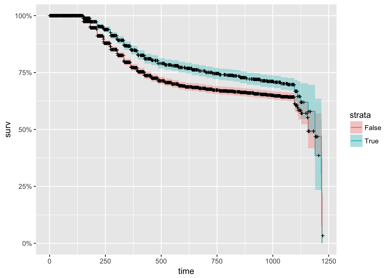
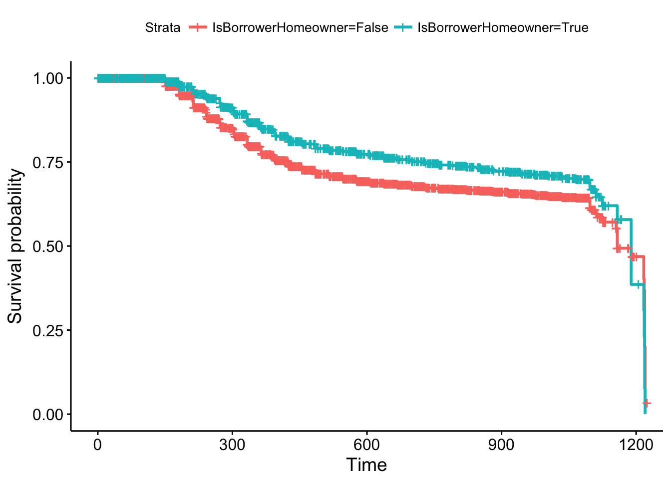
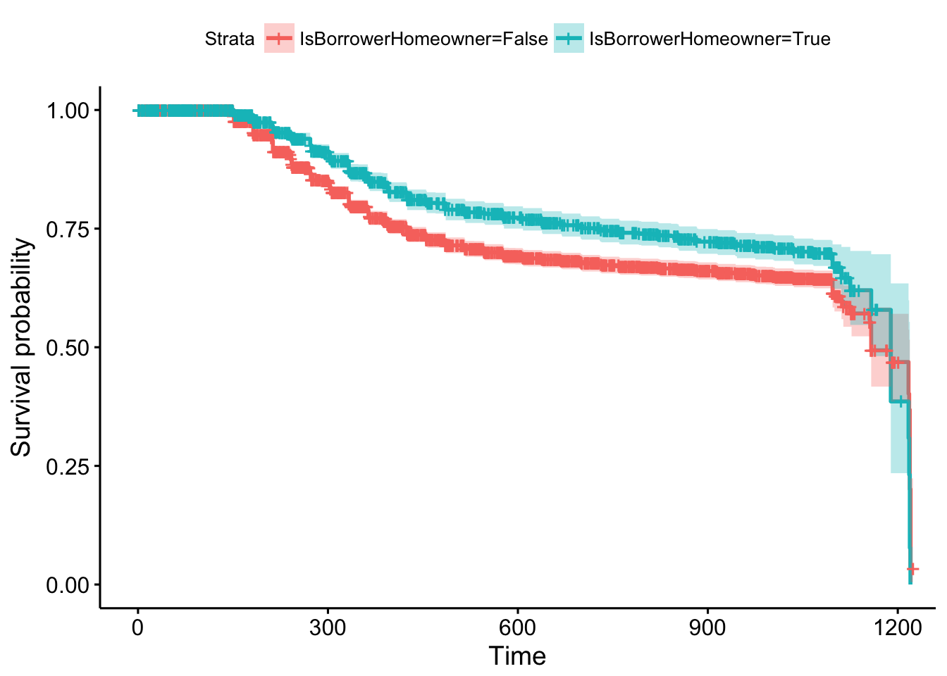
More beaitiful plots…
autoplot(model) #using ggplot2
survminer::ggsurvplot(model)
survminer::ggsurvplot(model, conf.int = TRUE)
References
Mantel, Nathan. 1966. “Evaluation of Survival Data and Two New Rank Order Statistics Arising in Its Consideration.” Cancer Chemotherapy Reports 50 (3): 163–70.
Peto, Richard, and Julian Peto. 1972. “Asymptotically Efficient Rank Invariant Test Procedures (with Discussion).” Journal of the Royal Statistical Society, Series A 135: 185–206.
Gehan, Edmund A. 1965. “A Generalized Wilcoxon Test for Comparing Arbitrarily Singly Censored Samples.” Biometrika 52. [Oxford University Press, Biometrika Trust]: 203–23. http://www.jstor.org/stable/2333825.
Mann, H. B., and D. R. Whitney. 1947. “On a Test of Whether One of Two Random Variables Is Stochastically Larger Than the Other.” Ann. Math. Statist. 18 (1). The Institute of Mathematical Statistics: 50–60. doi:10.1214/aoms/1177730491.
Kruskal, William H., and W. Allen Wallis. 1952. “Use of Ranks in One-Criterion Variance Analysis.” Journal of the American Statistical Association 47 (260). Taylor & Francis: 583–621. doi:10.1080/01621459.1952.10483441.
Tarone, Robert E., and James Ware. 1977. “On Distribution-Free Tests for Equality of Survival Distribution.” Biometrika 64: 156–60.